Imputation (Metabolomics example)#
In this notebook, we will showcase the acore functions for imputing data which are specific for metabolomics data analysis. Namely, we will go through imputation with zeros and half-minimum imputation.
For this, we will use a Diabetes example data set from this paper: Barranco-Altirriba M et al., 2025
This notebook refers to the acore.imputation_analysis module.
%pip install acore
Data Loading#
Load in your data and inspect the resulting dataframe. The example data set can be found
in example_data/DidacMauricio_hilic.
The data set has been filtered already, using the
acore.filter_metabolomics module. That means that
features with a lot of missingness have been filtered out already, meaning that the
features that are remaining have limited missingness and the data set is ready for the
imputation step.
data_path = (
    "https://raw.githubusercontent.com/Multiomics-Analytics-Group/acore/"
    "refs/heads/main/"
)
data_path = "../../example_data/DidacMauricio_hilic/DM_FIS2018_Hilic_pos_results2023_filtered.csv"
data_original = pd.read_csv(data_path, index_col=0)
data_original
| Qidx | SOIidx | rtmed | start | end | mass | MaxInt | formula | anot | AAA9485207 | ... | QC_35 | QC_36 | QC_37 | QC_38 | QC_39 | QC_40 | QC_41 | QC_42 | QC_43 | QC_44 | |
|---|---|---|---|---|---|---|---|---|---|---|---|---|---|---|---|---|---|---|---|---|---|
| 0 | 3 | 6 | 143.225 | 116.953 | 165.260 | 82.053 | 134,492.109 | [C4H6N2]+ | C4H5N2_M+H | 106,222.969 | ... | 117,823.602 | 122,279.500 | 120,513.508 | 119,803.422 | 114,791.906 | 124,753.789 | 128,157.016 | 115,411.750 | 133,331.281 | 124,152.578 |
| 1 | 4 | 7 | 330.747 | 313.125 | 373.976 | 82.065 | 67,051.617 | [C5H8N]+ | C5H7N_M+H | 40,187.371 | ... | 58,493.379 | 55,851.680 | 58,560.121 | 57,886.605 | 58,293.699 | 46,211.445 | 62,802.289 | 57,658.062 | 54,058.363 | 54,484.602 |
| 2 | 5 | 7 | 343.980 | 313.125 | 373.976 | 82.065 | 67,051.617 | [C5H8N]+ | C5H7N_M+H | 16,231.437 | ... | 25,015.951 | 21,309.277 | 20,180.580 | 19,609.604 | 25,462.301 | 24,354.287 | 30,869.357 | 17,454.047 | 22,235.070 | 18,160.814 |
| 3 | 8 | 14 | 329.952 | 315.544 | 343.132 | 84.081 | 192,073.984 | [C5H10N]+ | C5H9N_M+H | 112,320.398 | ... | 148,706.016 | 145,798.000 | 138,684.266 | 159,189.266 | 166,255.984 | 165,567.125 | 151,410.297 | 150,344.312 | 160,134.375 | 158,760.438 |
| 4 | 9 | 14 | 323.071 | 315.544 | 343.132 | 84.081 | 192,073.984 | [C5H10N]+ | C5H9N_M+H | 46,083.371 | ... | 93,403.664 | 102,219.703 | 101,832.156 | 104,895.648 | 154,315.234 | 135,517.156 | 134,795.859 | 130,498.227 | 124,771.242 | 126,280.156 |
| ... | ... | ... | ... | ... | ... | ... | ... | ... | ... | ... | ... | ... | ... | ... | ... | ... | ... | ... | ... | ... | ... |
| 1,997 | 2,541 | 2,363 | 299.617 | 290.000 | 312.500 | 892.654 | 3,486,662.000 | [C48H94NO11S]+ | C48H93NO11S_M+H | 137,733.500 | ... | 66,690.800 | 53,758.060 | 100,864.900 | 88,069.460 | 94,612.190 | 87,438.410 | 78,174.880 | 61,854.690 | 92,978.760 | 69,441.320 |
| 1,998 | 2,542 | 2,364 | 54.789 | 50.000 | 67.500 | 892.739 | 179,925.600 | [C57H98NO6]+ | C57H94O6_M+NH4 | 130,200.000 | ... | 190,497.800 | 173,043.300 | 57,476.910 | 174,392.000 | 47,625.360 | 135,338.900 | 154,609.500 | 179,258.000 | 171,145.200 | 161,171.100 |
| 1,999 | 2,543 | 2,365 | 54.782 | 50.000 | 67.500 | 894.755 | 488,985.200 | [C57H100NO6]+ | C57H96O6_M+NH4 | 468,793.800 | ... | 523,346.000 | 453,992.800 | 133,935.100 | 509,662.500 | 114,995.100 | 381,900.100 | 421,614.900 | 503,656.400 | 439,513.500 | 434,035.700 |
| 2,000 | 2,544 | 2,366 | 274.326 | 270.000 | 282.500 | 896.614 | 56,311.420 | [C51H88NNaO8P]+ | C51H88NO8P_M+Na | NaN | ... | 43,825.190 | 48,425.100 | 39,431.220 | 50,343.310 | 43,757.750 | 47,352.600 | 44,703.080 | 47,304.730 | 49,199.190 | 39,543.240 |
| 2,001 | 2,545 | 2,367 | 54.821 | 50.000 | 67.500 | 896.770 | 843,227.000 | [C57H102NO6]+ | C57H98O6_M+NH4 | 821,122.200 | ... | 998,584.700 | 897,026.200 | 235,440.700 | 809,741.600 | 178,420.900 | 678,957.200 | 785,135.600 | 895,259.400 | 788,261.100 | 768,748.800 |
2002 rows × 486 columns
In order to run our further analysis, including the filtering functions, we have to transform the data and remove metadata such as mass and retention time.
# first drop object columns, then transpose to keep columns numeric.
data = data_original.drop(
    ["Qidx", "SOIidx", "rtmed", "start", "end", "mass", "MaxInt", "formula", "anot"],
    axis=1,
).T
data
| 0 | 1 | 2 | 3 | 4 | 5 | 6 | 7 | 8 | 9 | ... | 1,992 | 1,993 | 1,994 | 1,995 | 1,996 | 1,997 | 1,998 | 1,999 | 2,000 | 2,001 | |
|---|---|---|---|---|---|---|---|---|---|---|---|---|---|---|---|---|---|---|---|---|---|
| AAA9485207 | 106,222.969 | 40,187.371 | 16,231.437 | 112,320.398 | 46,083.371 | 48,803.125 | 9,355.179 | 10,520.453 | 118,007.117 | 276,328.406 | ... | 80,973.820 | 46,157.050 | 49,622.580 | 231,180.200 | 6,403,619.000 | 137,733.500 | 130,200.000 | 468,793.800 | NaN | 821,122.200 |
| AAA9485216 | 132,690.734 | 82,426.359 | 24,345.967 | 84,265.992 | 73,903.742 | 43,815.148 | 15,694.467 | 6,981.189 | 144,795.078 | 6,585.585 | ... | 134,861.800 | 90,832.130 | 72,869.770 | 240,460.700 | 4,852,053.000 | 59,179.240 | 132,118.200 | 513,293.500 | NaN | 1,214,919.000 |
| AAA9485239 | 152,236.844 | 74,535.336 | 35,357.852 | 199,175.516 | 68,742.586 | 44,511.543 | 16,638.094 | 3,058.750 | 66,724.172 | 513,312.406 | ... | 85,438.980 | 63,371.030 | 49,218.960 | 310,655.100 | 2,619,595.000 | 72,289.910 | 160,829.900 | 518,888.200 | 35,597.220 | 1,092,635.000 |
| AAA9485258 | 113,827.773 | 51,309.215 | 20,640.715 | 271,096.281 | 41,593.598 | 61,431.602 | 15,303.128 | 6,524.716 | 254,299.859 | 517,436.312 | ... | 64,054.850 | 69,871.040 | 51,861.310 | 184,134.600 | 2,601,840.000 | 70,717.240 | 83,523.680 | 252,012.400 | NaN | 658,375.000 |
| AAA9485261 | 115,821.445 | 60,884.336 | 18,506.797 | 174,622.797 | 49,389.219 | 41,346.922 | 13,429.741 | 4,210.501 | 161,283.281 | 341,975.375 | ... | 191,401.000 | 114,394.600 | 98,023.710 | 359,151.000 | 2,767,868.000 | 150,113.300 | 143,107.200 | 463,635.800 | NaN | 1,099,109.000 |
| ... | ... | ... | ... | ... | ... | ... | ... | ... | ... | ... | ... | ... | ... | ... | ... | ... | ... | ... | ... | ... | ... |
| QC_40 | 124,753.789 | 46,211.445 | 24,354.287 | 165,567.125 | 135,517.156 | 52,733.680 | 19,532.146 | 7,451.286 | 146,865.938 | 362,608.625 | ... | 77,415.330 | 52,939.590 | 40,989.100 | 141,548.000 | 4,531,348.000 | 87,438.410 | 135,338.900 | 381,900.100 | 47,352.600 | 678,957.200 |
| QC_41 | 128,157.016 | 62,802.289 | 30,869.357 | 151,410.297 | 134,795.859 | 57,720.047 | 17,125.811 | 10,407.162 | 155,070.453 | 351,609.469 | ... | 70,159.380 | 89,829.210 | 46,564.210 | 172,408.800 | 4,375,519.000 | 78,174.880 | 154,609.500 | 421,614.900 | 44,703.080 | 785,135.600 |
| QC_42 | 115,411.750 | 57,658.062 | 17,454.047 | 150,344.312 | 130,498.227 | 50,533.473 | 18,608.479 | 9,215.572 | 173,242.469 | 352,352.438 | ... | 85,322.640 | 49,600.440 | 44,505.460 | 161,372.500 | 3,864,418.000 | 61,854.690 | 179,258.000 | 503,656.400 | 47,304.730 | 895,259.400 |
| QC_43 | 133,331.281 | 54,058.363 | 22,235.070 | 160,134.375 | 124,771.242 | 48,362.730 | 12,418.278 | 9,298.831 | 138,345.156 | 356,648.500 | ... | 78,372.000 | 54,991.750 | 53,880.830 | 145,470.600 | 3,730,628.000 | 92,978.760 | 171,145.200 | 439,513.500 | 49,199.190 | 788,261.100 |
| QC_44 | 124,152.578 | 54,484.602 | 18,160.814 | 158,760.438 | 126,280.156 | 46,164.520 | 18,341.426 | 9,914.410 | 158,816.812 | 353,626.719 | ... | 82,817.930 | 55,926.430 | 50,953.160 | 160,843.600 | 5,249,600.000 | 69,441.320 | 161,171.100 | 434,035.700 | 39,543.240 | 768,748.800 |
477 rows × 2002 columns
Check how much missingness there is in the data.
Total count of missing cells: 16289
Overall percentage of missingness: 1.705736611396989
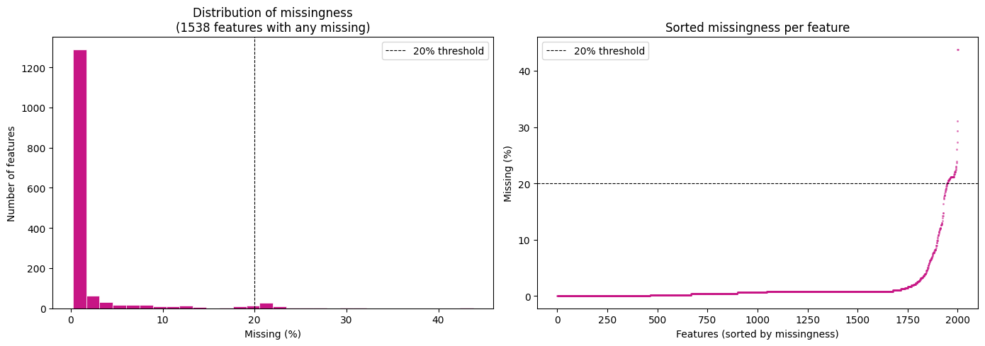
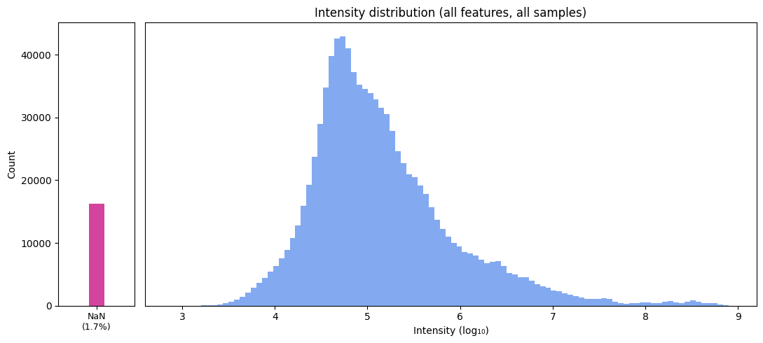
As we can see, overall, 1.7% of the dataset is missing. There are some features that have a lot of missing values, whereas most have very few.
Now that we have an overview, we can try two different methods of imputation.
Imputing with zeros#
In this method, which is commonly used in metabolomics and often automatically done by
preprocessing software like MetaboIgniter, all missing values get filled in with zeros.
This is done following the assumption of missing-not-at-random; that measurements may be missing not because they are truly absent in the biological sample but because they are for example below the limit of detection. Zero is then the lowest possible value that can be measured, and thus a reasonable imputation value for missing values.
Here, this method can be applied easily using the function
imputation_zeros().
Help on function imputation_zeros in module acore.imputation_analysis:

imputation_zeros(data: pandas.core.frame.DataFrame, on_cols: Optional[Iterable[str]] = None, on_rows: Optional[Iterable[str]] = None, drop_cols: Optional[Iterable[str]] = None)
    Replace missing values with zeros.

    :param data: DataFrame with samples as rows and features as columns.
    :param list on_cols: columns to fill with zeros. If `None`, all numeric columns are filled.
                         Non-numeric columns in "on_cols" will raise a TypeError.
    :param list on_rows: row index labels to restrict imputation to. If `None`, all rows are
                         imputed. Useful for imputing only a subset of samples (e.g. QCs,
                         blanks, controls) while leaving others untouched.
    :param list drop_cols: columns to permanently drop before imputation. If a column
                           appears in both "on_cols" and "drop_cols" it will be dropped
                           and a warning is emitted.
    :return: DataFrame with missing values in the target columns replaced by zero.

    Example:

        result = imputation_zeros(data, on_cols=['featureA', 'featureB'])
        result = imputation_zeros(data, on_rows=['QC1', 'QC2', 'blank1'])
data_imputed_zeros = imputation_zeros(data=data)
Total count of missing cells: 0
Overall percentage of missingness: 0.0

SUMMARY of imputation changes:
Total values      : 954,954
Missing before    : 16,289  (1.7%)
Missing after     : 0  (0.0%)
Features affected : 1538 / 2002
Samples affected  : 436 / 477
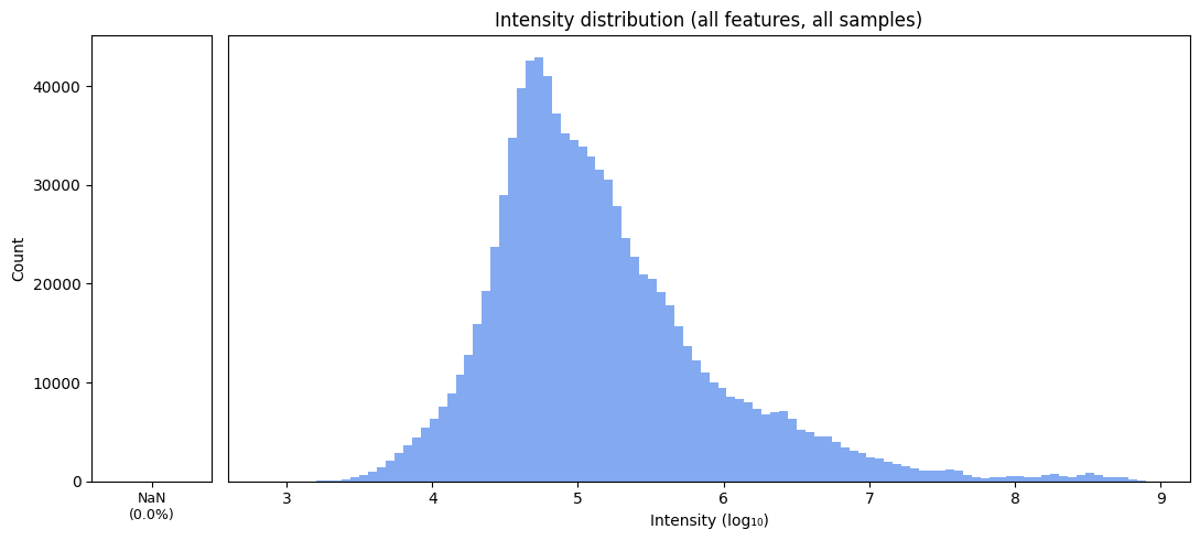
We have imputed all of our missing values with zeros.
Imputation with half minimum#
This method is also widely used across the metabolomics community. Here, missing values are imputed with half of the minimum value that has been recorded across the data set.
This is done following the assumption of missing-not-at-random; that measurements may be missing not because they are truly absent in the biological sample but because they are for example below the limit of detection.
Here, in acore, the function
imputation_half_minimum() is used
for this.
Help on function imputation_half_minimum in module acore.imputation_analysis:

imputation_half_minimum(data: pandas.core.frame.DataFrame, on_cols: Optional[Iterable[str]] = None, on_rows: Optional[Iterable[str]] = None, drop_cols: Optional[Iterable[str]] = None)
    Replace missing values with half the per-column minimum of observed values.

    :param data: DataFrame with samples as rows and features as columns.
    :param list on_cols: columns to impute. If None, all numeric columns are used.
                         Non-numeric columns in ``on_cols`` will raise a TypeError.
    :param list on_rows: row index labels to restrict imputation to. If None, all rows are
                         imputed. When provided, the per-column minimum is also computed
                         from only those rows, so each subset gets its own half-minimum
                         (e.g. blanks are imputed with half the blank-minimum).
    :param list drop_cols: columns to permanently drop before imputation. If a column
                           appears in both ``on_cols`` and ``drop_cols`` it will be dropped
                           and a warning is emitted.
    :return: DataFrame with missing values replaced by half the per-column minimum.

    Example::

        result = imputation_half_minimum(data, on_cols=['featureA', 'featureB'])
        result = imputation_half_minimum(data, on_rows=['blank1', 'blank2'])
data_imputed_hm = imputation_half_minimum(data)
Total count of missing cells: 0
Overall percentage of missingness: 0.0

SUMMARY of imputation changes:
Total values      : 954,954
Missing before    : 16,289  (1.7%)
Missing after     : 0  (0.0%)
Features affected : 1538 / 2002
Samples affected  : 436 / 477
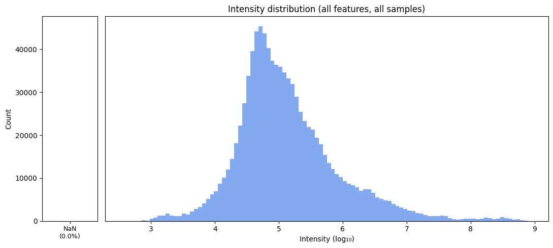
Again, we can see that after imputation, no missing values are left in our data.