

Metabolomics drift correction#
Within-batch correction of metabolomics data. This notebook shows how to correct for instrumental drift based on pooled QC data samples.
1. LOESS smoothing-based drift correction#
First, let’s load our packages, including acore.
%pip install acore
import matplotlib.pyplot as plt
import numpy as np
import pandas as pd
from sklearn.decomposition import PCA
from sklearn.preprocessing import StandardScaler

from acore import drift_correction as dc
Load in data#
We will use some example data that can be found in this repo.
data_path = (
    "https://raw.githubusercontent.com/Multiomics-Analytics-Group/acore/"
    "refs/heads/main/"
)

df_original = pd.read_csv(
    "../../example_data/DidacMauricio_hilic/DM_FIS2018_Hilic_pos_results2023_filled_imputed.csv",
    index_col=0,
)
This is what the data frame, an intensity table, looks like.
df_original
| Qidx | SOIidx | rtmed | start | end | mass | MaxInt | formula | anot | AAA9485207 | ... | QC_35 | QC_36 | QC_37 | QC_38 | QC_39 | QC_40 | QC_41 | QC_42 | QC_43 | QC_44 | |
|---|---|---|---|---|---|---|---|---|---|---|---|---|---|---|---|---|---|---|---|---|---|
| 0 | 1 | 1 | 60.544 | 45.000 | 72.500 | 81.070 | 160,840.953 | [C6H9]+ | C6H8_M+H | 279,488.531 | ... | 142,100.734 | 129,631.148 | 110,443.422 | 157,871.062 | 535,311.375 | 334,133.656 | 339,973.344 | 317,506.188 | 294,083.344 | 234,717.266 |
| 1 | 2 | 4 | 172.568 | 161.439 | 191.635 | 82.053 | 98,153.547 | [C4H6N2]+ | C4H5N2_M+H | 73,170.344 | ... | 72,917.398 | 73,738.812 | 65,597.875 | 78,216.859 | 70,257.375 | 73,489.242 | 60,233.695 | 70,798.312 | 69,802.516 | 74,212.203 |
| 2 | 3 | 6 | 143.225 | 116.953 | 165.260 | 82.053 | 134,492.109 | [C4H6N2]+ | C4H5N2_M+H | 106,222.969 | ... | 117,823.602 | 122,279.500 | 120,513.508 | 119,803.422 | 114,791.906 | 124,753.789 | 128,157.016 | 115,411.750 | 133,331.281 | 124,152.578 |
| 3 | 4 | 7 | 330.747 | 313.125 | 373.976 | 82.065 | 67,051.617 | [C5H8N]+ | C5H7N_M+H | 40,187.371 | ... | 58,493.379 | 55,851.680 | 58,560.121 | 57,886.605 | 58,293.699 | 46,211.445 | 62,802.289 | 57,658.062 | 54,058.363 | 54,484.602 |
| 4 | 5 | 7 | 343.980 | 313.125 | 373.976 | 82.065 | 67,051.617 | [C5H8N]+ | C5H7N_M+H | 16,231.437 | ... | 25,015.951 | 21,309.277 | 20,180.580 | 19,609.604 | 25,462.301 | 24,354.287 | 30,869.357 | 17,454.047 | 22,235.070 | 18,160.814 |
| ... | ... | ... | ... | ... | ... | ... | ... | ... | ... | ... | ... | ... | ... | ... | ... | ... | ... | ... | ... | ... | ... |
| 2,539 | 2,540 | 2,363 | 290.896 | 290.000 | 312.500 | 892.654 | 3,486,662.000 | [C48H94NO11S]+ | C48H93NO11S_M+H | 6,403,619.000 | ... | 4,217,977.000 | 3,872,732.000 | 3,356,819.000 | 3,444,360.000 | 3,641,683.000 | 4,531,348.000 | 4,375,519.000 | 3,864,418.000 | 3,730,628.000 | 5,249,600.000 |
| 2,540 | 2,541 | 2,363 | 299.617 | 290.000 | 312.500 | 892.654 | 3,486,662.000 | [C48H94NO11S]+ | C48H93NO11S_M+H | 137,733.500 | ... | 66,690.800 | 53,758.060 | 100,864.900 | 88,069.460 | 94,612.190 | 87,438.410 | 78,174.880 | 61,854.690 | 92,978.760 | 69,441.320 |
| 2,541 | 2,542 | 2,364 | 54.789 | 50.000 | 67.500 | 892.739 | 179,925.600 | [C57H98NO6]+ | C57H94O6_M+NH4 | 130,200.000 | ... | 190,497.800 | 173,043.300 | 57,476.910 | 174,392.000 | 47,625.360 | 135,338.900 | 154,609.500 | 179,258.000 | 171,145.200 | 161,171.100 |
| 2,542 | 2,543 | 2,365 | 54.782 | 50.000 | 67.500 | 894.755 | 488,985.200 | [C57H100NO6]+ | C57H96O6_M+NH4 | 468,793.800 | ... | 523,346.000 | 453,992.800 | 133,935.100 | 509,662.500 | 114,995.100 | 381,900.100 | 421,614.900 | 503,656.400 | 439,513.500 | 434,035.700 |
| 2,544 | 2,545 | 2,367 | 54.821 | 50.000 | 67.500 | 896.770 | 843,227.000 | [C57H102NO6]+ | C57H98O6_M+NH4 | 821,122.200 | ... | 998,584.700 | 897,026.200 | 235,440.700 | 809,741.600 | 178,420.900 | 678,957.200 | 785,135.600 | 895,259.400 | 788,261.100 | 768,748.800 |
2287 rows × 486 columns
In order to run our further analysis, including the filtering functions, we have to transform the data and remove metadata such as mass and retention time.
df = df_original.T
df = df.drop(
    ["Qidx", "SOIidx", "rtmed", "start", "end", "mass", "MaxInt", "formula", "anot"]
)
| 0 | 1 | 2 | 3 | 4 | 5 | 6 | 7 | 8 | 9 | ... | 2,534 | 2,535 | 2,536 | 2,537 | 2,538 | 2,539 | 2,540 | 2,541 | 2,542 | 2,544 | |
|---|---|---|---|---|---|---|---|---|---|---|---|---|---|---|---|---|---|---|---|---|---|
| AAA9485207 | 279,488.531 | 73,170.344 | 106,222.969 | 40,187.371 | 16,231.437 | 211,807.094 | 319,754.562 | 112,320.398 | 46,083.371 | 48,803.125 | ... | 82,146.870 | 80,973.820 | 46,157.050 | 49,622.580 | 231,180.200 | 6,403,619.000 | 137,733.500 | 130,200.000 | 468,793.800 | 821,122.200 |
| AAA9485216 | 247,458.016 | 86,581.648 | 132,690.734 | 82,426.359 | 24,345.967 | 12,622.342 | 389,471.938 | 84,265.992 | 73,903.742 | 43,815.148 | ... | 148,114.400 | 134,861.800 | 90,832.130 | 72,869.770 | 240,460.700 | 4,852,053.000 | 59,179.240 | 132,118.200 | 513,293.500 | 1,214,919.000 |
| AAA9485239 | 99,304.359 | 93,201.195 | 152,236.844 | 74,535.336 | 35,357.852 | 7,571.239 | 417,576.844 | 199,175.516 | 68,742.586 | 44,511.543 | ... | 95,990.200 | 85,438.980 | 63,371.030 | 49,218.960 | 310,655.100 | 2,619,595.000 | 72,289.910 | 160,829.900 | 518,888.200 | 1,092,635.000 |
| AAA9485258 | 119,563.797 | 72,692.320 | 113,827.773 | 51,309.215 | 20,640.715 | 259,447.391 | 340,227.594 | 271,096.281 | 41,593.598 | 61,431.602 | ... | 83,902.570 | 64,054.850 | 69,871.040 | 51,861.310 | 184,134.600 | 2,601,840.000 | 70,717.240 | 83,523.680 | 252,012.400 | 658,375.000 |
| AAA9485261 | 191,762.188 | 64,645.020 | 115,821.445 | 60,884.336 | 18,506.797 | 235,303.953 | 320,328.281 | 174,622.797 | 49,389.219 | 41,346.922 | ... | 221,212.200 | 191,401.000 | 114,394.600 | 98,023.710 | 359,151.000 | 2,767,868.000 | 150,113.300 | 143,107.200 | 463,635.800 | 1,099,109.000 |
| ... | ... | ... | ... | ... | ... | ... | ... | ... | ... | ... | ... | ... | ... | ... | ... | ... | ... | ... | ... | ... | ... |
| QC_40 | 334,133.656 | 73,489.242 | 124,753.789 | 46,211.445 | 24,354.287 | 246,895.516 | 399,774.781 | 165,567.125 | 135,517.156 | 52,733.680 | ... | 81,523.700 | 77,415.330 | 52,939.590 | 40,989.100 | 141,548.000 | 4,531,348.000 | 87,438.410 | 135,338.900 | 381,900.100 | 678,957.200 |
| QC_41 | 339,973.344 | 60,233.695 | 128,157.016 | 62,802.289 | 30,869.357 | 254,287.641 | 407,853.812 | 151,410.297 | 134,795.859 | 57,720.047 | ... | 62,895.500 | 70,159.380 | 89,829.210 | 46,564.210 | 172,408.800 | 4,375,519.000 | 78,174.880 | 154,609.500 | 421,614.900 | 785,135.600 |
| QC_42 | 317,506.188 | 70,798.312 | 115,411.750 | 57,658.062 | 17,454.047 | 264,687.438 | 407,221.000 | 150,344.312 | 130,498.227 | 50,533.473 | ... | 73,050.480 | 85,322.640 | 49,600.440 | 44,505.460 | 161,372.500 | 3,864,418.000 | 61,854.690 | 179,258.000 | 503,656.400 | 895,259.400 |
| QC_43 | 294,083.344 | 69,802.516 | 133,331.281 | 54,058.363 | 22,235.070 | 269,192.375 | 394,239.344 | 160,134.375 | 124,771.242 | 48,362.730 | ... | 71,588.570 | 78,372.000 | 54,991.750 | 53,880.830 | 145,470.600 | 3,730,628.000 | 92,978.760 | 171,145.200 | 439,513.500 | 788,261.100 |
| QC_44 | 234,717.266 | 74,212.203 | 124,152.578 | 54,484.602 | 18,160.814 | 261,814.906 | 412,434.000 | 158,760.438 | 126,280.156 | 46,164.520 | ... | 78,520.450 | 82,817.930 | 55,926.430 | 50,953.160 | 160,843.600 | 5,249,600.000 | 69,441.320 | 161,171.100 | 434,035.700 | 768,748.800 |
477 rows × 2287 columns
We also have data that contains the order in which our samples were run. This information is crucial for the drift correction algorithm; it cannot be performed without it.
The data needs to contain the columns File Name and Sample ID, referring to the
name of the sample and the index of the sample, meaning the order in which the samples
were run.
Note: If you do not have metadata that contains the order in which samples and QCs were run, you can use the second method explained in this notebook, CPCA.
sample_order = pd.read_csv(
    "../../example_data/DidacMauricio_hilic/DidacMauricio_hilic_pos_injectionorder.csv"
)
sample_order["File Name"] = sample_order["SampleName"]
sample_order["Sample ID"] = sample_order["injectionOrder"]

sample_order
| SampleName | measureTime | injectionOrder | File Name | Sample ID | |
|---|---|---|---|---|---|
| 0 | Bi_1 | 2021-07-19 13:51:34 | 1 | Bi_1 | 1 |
| 1 | Bi_2 | 2021-07-19 14:05:49 | 2 | Bi_2 | 2 |
| 2 | QC_00 | 2021-07-19 14:20:04 | 3 | QC_00 | 3 |
| 3 | QC_01 | 2021-07-19 14:34:20 | 4 | QC_01 | 4 |
| 4 | QC_02 | 2021-07-19 14:48:36 | 5 | QC_02 | 5 |
| ... | ... | ... | ... | ... | ... |
| 472 | AAA9516105 | 2021-07-24 06:04:54 | 473 | AAA9516105 | 473 |
| 473 | QC_43 | 2021-07-24 06:19:11 | 474 | QC_43 | 474 |
| 474 | QC_44 | 2021-07-24 06:33:27 | 475 | QC_44 | 475 |
| 475 | Bf_1 | 2021-07-24 06:47:43 | 476 | Bf_1 | 476 |
| 476 | Bf_2 | 2021-07-24 07:01:57 | 477 | Bf_2 | 477 |
477 rows × 5 columns
Run drift correction with LOESS smoothing#
We can now correct our data for experimental drift.
With the acore LOESS drift-correction function, a LOESS (locally estimated regression) smoother is applied separately to the features in the data to model slow temporal trends, and the resulting smooth trend is used to correct the data.
Before the function estimation and correction, the data can filtered, to remove features that have too many missing values in the QC samples.
First, we can create a dictionary for our sample names, ordering them into groups, to make the upcoming function call easier.
column_list = list(df_original.columns.values)
sample_cols = []
qc_cols = []
for col in column_list:
    if col.startswith("AAA"):
        sample_cols.append(col)
    elif col.startswith("QC"):
        qc_cols.append(col)
Now, are sample column names are summarised in the sample_cols variable:
sample_cols
Our columns corresponding to QC data are saved in the qc_cols variable:
qc_cols
Now we can run the drift correction, using the acore run_loess_drift_correction
function.
Note: For this demonstration, we will use the parameter always_use_default, so that the leave-one-out cross validation, during which the best smoothing parameter for the curve is determined, is skipped. This is just for efficiency purposes; so that this does not take too long to load. However, it is recommended to not use this option, so that the best parameter can be determined for the curve of every feature.
Help on function run_loess_drift_correction in module acore.drift_correction.loess_drift_correction:

run_loess_drift_correction(data, qc_rows, sample_rows, sample_order: pandas.core.frame.DataFrame, filter_percent: float = None, qc_min_threshold: int = 4, always_use_default=False, default=0.75)
    Perform QC-based drift correction across multiple features using
    LOESS regression and spline interpolation.

    For each feature:
    1. Extract QC intensities and corresponding injection order.
    2. Optionally filter features based on QC completeness.
    3. Compute QC relative standard deviation (RSD).
    4. If sufficient QC points exist, estimate a drift curve using
       `qc_rlsc_loess`, finding the best alpha smoothing span
       with leave-one-out cross validation (LOOCV).
    5. Normalize all intensities by dividing by the drift curve and
       scaling to the QC median.
    6. Record drift parameters and correction metadata.

    Parameters
    ----------
    data : pandas.DataFrame
        Input intensity matrix with samples as rows and features as columns.
    qc_rows : list of str
        Row indices corresponding to QC injections.
    sample_rows : list of str
        Row indices corresponding to biological samples.
    sample_order : pandas.DataFrame
        Table mapping file names to injection order. Must contain
        columns "File Name" and "Sample ID". Sample ID must be
        numeric.
    filter_percent : float, optional
        Minimum proportion of QC values that must be non-missing for
        a feature to be retained (e.g., 0.6 means at least 60% of QCs
        must be present).
    qc_min_threshold : int, optional
        Minimum number of QC values required to perform drift
        correction. Features with fewer QCs are returned uncorrected.
    always_use_default: bool, optional
        If True, LOOCV is skipped and `default` is used for the smoothing span.
        This option is less computationally heavy.
    default : float, optional
        Default alpha to use when `always_use_default=True` or when LOOCV fails.
        Defaults to 0.75.

    Returns
    -------
    corrected_df : pandas.DataFrame
        Full input DataFrame with corrected values applied to
        sample_rows + qc_rows. Rows outside those arguments are
        returned unchanged. Features that fail QC requirements are
        returned unchanged.
    correction_info : dict
        Dictionary keyed by feature name, containing:
        - 'alpha': selected LOESS alpha (or None if skipped)
        - 'drift_curve': the evaluated drift correction vector
        - 'y_qc': QC intensities used
        - 'x_qc': QC injection orders
        - 'rsd_qc': QC relative standard deviation
        - 'median': QC median intensity (used for scaling)
        - 'y_all': original intensities
        - 'status': "corrected", "skipped_due_to_few_qcs", or error note

    Notes
    -----
    - Features with insufficient QC points are not corrected.
    - High QC RSD (>20%) is flagged but does not prevent correction.
    - Drift correction rescales intensities so that QC medians remain
      unchanged.
    - Sample names in `data` and `sample_order` must match exactly.
corrected_df, correction_info = dc.run_loess_drift_correction(
    df,
    qc_cols,
    sample_cols,
    sample_order=sample_order,
    filter_percent=0.5,
    always_use_default=True,
)
Explanation of the parameters chosen:
filter_percentis the minimum percentage of values that must be present for this feature to be retained. If the percentage of non-missing is below this, the feature will be filtered out. If this parameter is set to “None”, no filtering will be done. In this case, the filter_percent parameter does not do anything, as the data is already imputed and there are no missing values in the QCs.always_use_defaultdisables the leave-one-out cross validation which calculates the ideal smoothing parameter for the LOESS curve for every feature. It will speed up the computation, but the curve which decides the value correction is less optimal.default(not used here) changes the default smoothing value. If the parameter is
not used, the default is 0.75. The default smoothing value is either used ifalways_use_default=True, or if no better smoothing parameter can be found during leave-one-out cross validation.
Now we can inspect our results. First, the corrected output dataframe.
| 0 | 1 | 2 | 3 | 4 | 5 | 6 | 7 | 8 | 9 | ... | 2,534 | 2,535 | 2,536 | 2,537 | 2,538 | 2,539 | 2,540 | 2,541 | 2,542 | 2,544 | |
|---|---|---|---|---|---|---|---|---|---|---|---|---|---|---|---|---|---|---|---|---|---|
| AAA9485207 | 170,751.900 | 74,733.789 | 102,226.405 | 40,643.193 | 17,407.179 | 207,850.329 | 301,741.759 | 122,012.671 | 46,842.939 | 49,591.009 | ... | 75,598.663 | 71,502.506 | 42,705.434 | 43,458.397 | 215,794.742 | 5,679,763.408 | 145,900.211 | 131,000.095 | 465,222.264 | 765,961.103 |
| AAA9485216 | 254,972.445 | 84,599.084 | 132,040.201 | 81,751.376 | 23,178.037 | 13,570.560 | 475,861.616 | 77,889.100 | 74,396.454 | 43,084.318 | ... | 149,558.074 | 149,252.662 | 89,124.808 | 72,306.254 | 249,371.922 | 4,910,196.789 | 63,632.247 | 139,196.065 | 548,226.926 | 1,284,688.374 |
| AAA9485239 | 105,650.309 | 88,336.415 | 149,311.684 | 73,415.302 | 32,831.615 | 8,150.034 | 507,872.985 | 181,674.039 | 72,859.812 | 43,520.085 | ... | 99,260.097 | 98,291.891 | 60,520.171 | 47,363.989 | 318,079.391 | 2,647,962.764 | 79,815.076 | 166,784.045 | 541,498.896 | 1,122,427.204 |
| AAA9485258 | 141,472.575 | 63,427.966 | 106,948.841 | 49,569.608 | 17,890.650 | 281,878.555 | 404,315.506 | 237,912.047 | 52,412.441 | 58,980.814 | ... | 93,657.648 | 83,965.724 | 61,541.640 | 45,676.443 | 181,279.890 | 2,620,000.022 | 84,364.087 | 82,649.318 | 246,072.506 | 623,095.027 |
| AAA9485261 | 168,001.076 | 70,318.948 | 116,960.462 | 61,511.168 | 19,872.293 | 251,266.323 | 340,996.938 | 182,178.869 | 46,781.756 | 41,506.735 | ... | 184,149.858 | 166,209.985 | 107,600.799 | 92,958.519 | 336,225.782 | 2,594,623.689 | 144,606.352 | 149,851.946 | 492,523.008 | 1,137,484.580 |
| ... | ... | ... | ... | ... | ... | ... | ... | ... | ... | ... | ... | ... | ... | ... | ... | ... | ... | ... | ... | ... | ... |
| QC_40 | 205,485.696 | 75,163.543 | 120,175.910 | 46,730.876 | 26,122.635 | 242,719.115 | 377,942.724 | 179,732.499 | 137,576.799 | 53,565.458 | ... | 74,795.591 | 68,295.325 | 48,961.170 | 35,936.651 | 132,050.733 | 4,022,401.965 | 92,399.577 | 136,253.218 | 379,418.707 | 634,454.149 |
| QC_41 | 203,188.136 | 61,241.011 | 122,943.150 | 63,540.061 | 33,088.069 | 248,059.085 | 382,615.399 | 164,834.093 | 137,556.507 | 58,724.437 | ... | 58,505.657 | 62,169.680 | 83,238.874 | 40,640.780 | 161,296.257 | 3,870,973.303 | 83,490.771 | 155,264.598 | 416,902.656 | 728,309.185 |
| QC_42 | 184,813.193 | 71,599.643 | 110,301.340 | 58,370.767 | 18,697.821 | 256,398.299 | 379,464.207 | 164,075.895 | 133,718.503 | 51,490.957 | ... | 68,901.645 | 75,972.002 | 46,061.444 | 38,701.025 | 151,468.529 | 3,409,242.520 | 66,731.838 | 179,643.882 | 496,034.602 | 825,262.125 |
| QC_43 | 166,722.545 | 70,228.397 | 126,958.386 | 54,767.289 | 23,808.660 | 258,972.175 | 365,043.498 | 175,160.016 | 128,289.958 | 49,356.198 | ... | 68,540.946 | 70,166.545 | 51,196.168 | 46,699.476 | 137,077.894 | 3,282,893.947 | 101,360.384 | 171,183.195 | 431,245.208 | 722,368.417 |
| QC_44 | 132,774.939 | 74,633.348 | 118,182.415 | 55,202.886 | 19,445.454 | 251,731.787 | 381,694.940 | 173,688.920 | 129,874.693 | 47,119.080 | ... | 75,275.158 | 74,182.938 | 52,077.927 | 44,150.561 | 151,617.540 | 4,618,642.405 | 75,767.913 | 161,181.787 | 425,742.116 | 704,153.537 |
477 rows × 2287 columns
We can also look further into the correction_info object, to see the parameters that were chosen for each feature.
For example, let’s check the parameters used for the 200th feature.
print(correction_info[200])
Plot an example curve for one feature#
We can also plot an example feature, to see how the values have changed and what the LOESS curve would look like for the data of this feature.
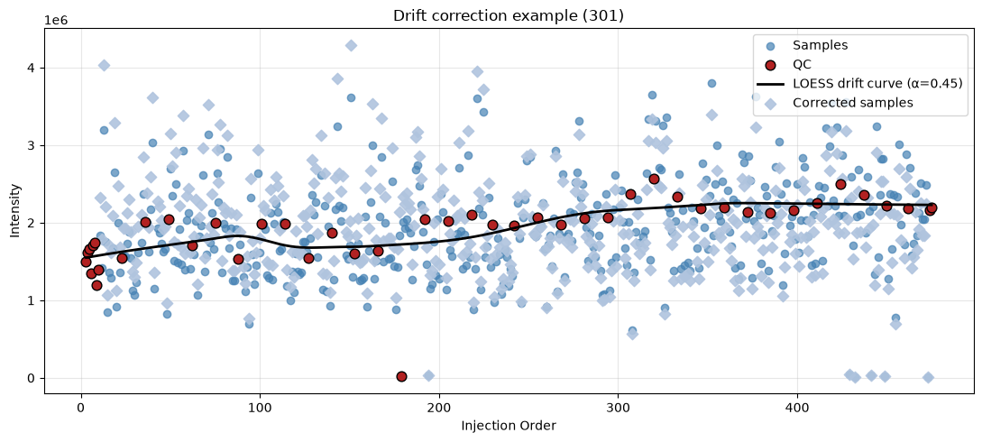
In this plot, we can see all of the data points of this feature, ordered by the injection time. The red points are our QC samples, so we can see whether there was any instrumental drift over time. The LOESS curve is also calculated, with the smoothing value alpha chosen with leave-one-out cross validation, just like in the run_drift_correction function.
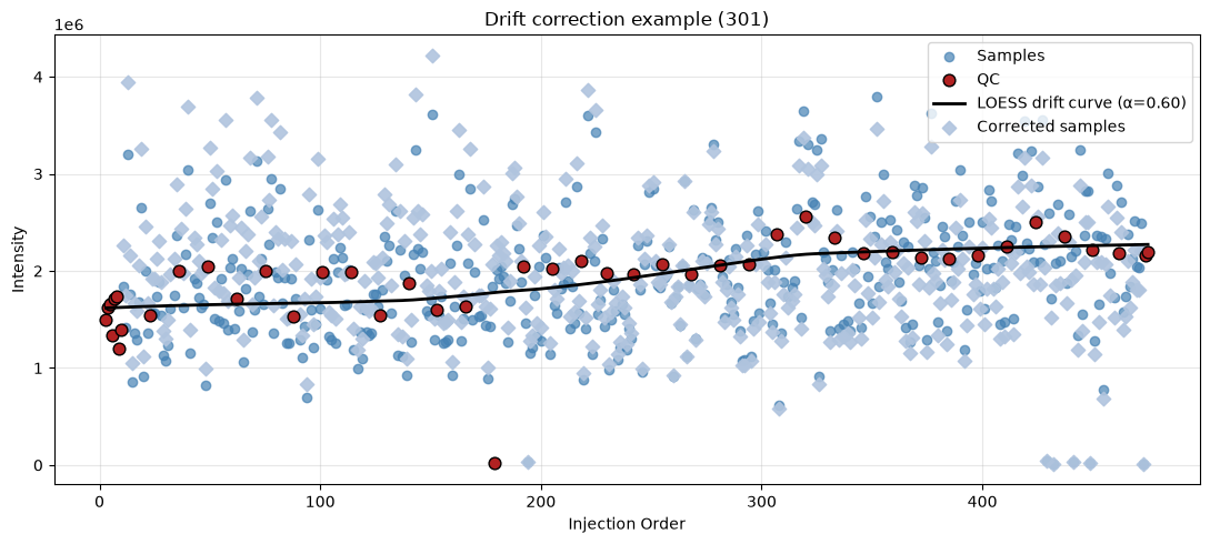
Alternative values for the smoothing parameter alpha can be tested by adding the argument “alpha” and choosing a value, just like in the example below.
2. Common Principal Components Analysis-based drift correction#
We can also use another method for correcting drift which is based on Common Principal Components Analysis (CPCA). This method is based on common principal components in defined groups of the data. It assumes that when calculating common principal components of QC samples, the drift contribution can be identified as the direction capturing maximum variance that simultaneously diagonalizes the covariance matrices of a set of classes.
Therefore, the variability in the identified direction can be explained as caused by experimental drift and subtracted from all samples.
Let’s use different example data for demonstrating this method.
Load in data#
# Load data
df_original = pd.read_csv(
    "../../example_data/DidacMauricio_hilic/DM_FIS2018_Hilic_pos_results2023_filled_imputed.csv",
    index_col=0,
)

df = df_original.T
df = df.drop(
    ["Qidx", "SOIidx", "rtmed", "start", "end", "mass", "MaxInt", "formula", "anot"]
)

# Define sample columns and qc columns
collist = list(df_original.columns.values)
sample_cols = []
qc_cols = []
for col in collist:
    if col.startswith("AAA"):
        sample_cols.append(col)
    elif col.startswith("QC"):
        qc_cols.append(col)
df
| 0 | 1 | 2 | 3 | 4 | 5 | 6 | 7 | 8 | 9 | ... | 2,534 | 2,535 | 2,536 | 2,537 | 2,538 | 2,539 | 2,540 | 2,541 | 2,542 | 2,544 | |
|---|---|---|---|---|---|---|---|---|---|---|---|---|---|---|---|---|---|---|---|---|---|
| AAA9485207 | 279,488.531 | 73,170.344 | 106,222.969 | 40,187.371 | 16,231.437 | 211,807.094 | 319,754.562 | 112,320.398 | 46,083.371 | 48,803.125 | ... | 82,146.870 | 80,973.820 | 46,157.050 | 49,622.580 | 231,180.200 | 6,403,619.000 | 137,733.500 | 130,200.000 | 468,793.800 | 821,122.200 |
| AAA9485216 | 247,458.016 | 86,581.648 | 132,690.734 | 82,426.359 | 24,345.967 | 12,622.342 | 389,471.938 | 84,265.992 | 73,903.742 | 43,815.148 | ... | 148,114.400 | 134,861.800 | 90,832.130 | 72,869.770 | 240,460.700 | 4,852,053.000 | 59,179.240 | 132,118.200 | 513,293.500 | 1,214,919.000 |
| AAA9485239 | 99,304.359 | 93,201.195 | 152,236.844 | 74,535.336 | 35,357.852 | 7,571.239 | 417,576.844 | 199,175.516 | 68,742.586 | 44,511.543 | ... | 95,990.200 | 85,438.980 | 63,371.030 | 49,218.960 | 310,655.100 | 2,619,595.000 | 72,289.910 | 160,829.900 | 518,888.200 | 1,092,635.000 |
| AAA9485258 | 119,563.797 | 72,692.320 | 113,827.773 | 51,309.215 | 20,640.715 | 259,447.391 | 340,227.594 | 271,096.281 | 41,593.598 | 61,431.602 | ... | 83,902.570 | 64,054.850 | 69,871.040 | 51,861.310 | 184,134.600 | 2,601,840.000 | 70,717.240 | 83,523.680 | 252,012.400 | 658,375.000 |
| AAA9485261 | 191,762.188 | 64,645.020 | 115,821.445 | 60,884.336 | 18,506.797 | 235,303.953 | 320,328.281 | 174,622.797 | 49,389.219 | 41,346.922 | ... | 221,212.200 | 191,401.000 | 114,394.600 | 98,023.710 | 359,151.000 | 2,767,868.000 | 150,113.300 | 143,107.200 | 463,635.800 | 1,099,109.000 |
| ... | ... | ... | ... | ... | ... | ... | ... | ... | ... | ... | ... | ... | ... | ... | ... | ... | ... | ... | ... | ... | ... |
| QC_40 | 334,133.656 | 73,489.242 | 124,753.789 | 46,211.445 | 24,354.287 | 246,895.516 | 399,774.781 | 165,567.125 | 135,517.156 | 52,733.680 | ... | 81,523.700 | 77,415.330 | 52,939.590 | 40,989.100 | 141,548.000 | 4,531,348.000 | 87,438.410 | 135,338.900 | 381,900.100 | 678,957.200 |
| QC_41 | 339,973.344 | 60,233.695 | 128,157.016 | 62,802.289 | 30,869.357 | 254,287.641 | 407,853.812 | 151,410.297 | 134,795.859 | 57,720.047 | ... | 62,895.500 | 70,159.380 | 89,829.210 | 46,564.210 | 172,408.800 | 4,375,519.000 | 78,174.880 | 154,609.500 | 421,614.900 | 785,135.600 |
| QC_42 | 317,506.188 | 70,798.312 | 115,411.750 | 57,658.062 | 17,454.047 | 264,687.438 | 407,221.000 | 150,344.312 | 130,498.227 | 50,533.473 | ... | 73,050.480 | 85,322.640 | 49,600.440 | 44,505.460 | 161,372.500 | 3,864,418.000 | 61,854.690 | 179,258.000 | 503,656.400 | 895,259.400 |
| QC_43 | 294,083.344 | 69,802.516 | 133,331.281 | 54,058.363 | 22,235.070 | 269,192.375 | 394,239.344 | 160,134.375 | 124,771.242 | 48,362.730 | ... | 71,588.570 | 78,372.000 | 54,991.750 | 53,880.830 | 145,470.600 | 3,730,628.000 | 92,978.760 | 171,145.200 | 439,513.500 | 788,261.100 |
| QC_44 | 234,717.266 | 74,212.203 | 124,152.578 | 54,484.602 | 18,160.814 | 261,814.906 | 412,434.000 | 158,760.438 | 126,280.156 | 46,164.520 | ... | 78,520.450 | 82,817.930 | 55,926.430 | 50,953.160 | 160,843.600 | 5,249,600.000 | 69,441.320 | 161,171.100 | 434,035.700 | 768,748.800 |
477 rows × 2287 columns
Seeing as this method is based on calculating principal components, as with PCA, there must not be any missing data.
We will therefore first calculate missingness (NAs).
We need to check for missing values in both the sample columns and the QC columns.
There is no missingness. We can proceed with the CPCA drift correction.
Visualise non-corrected data#
Now that we know we can proceed, let’s visualise our data before drift correction with a PCA.
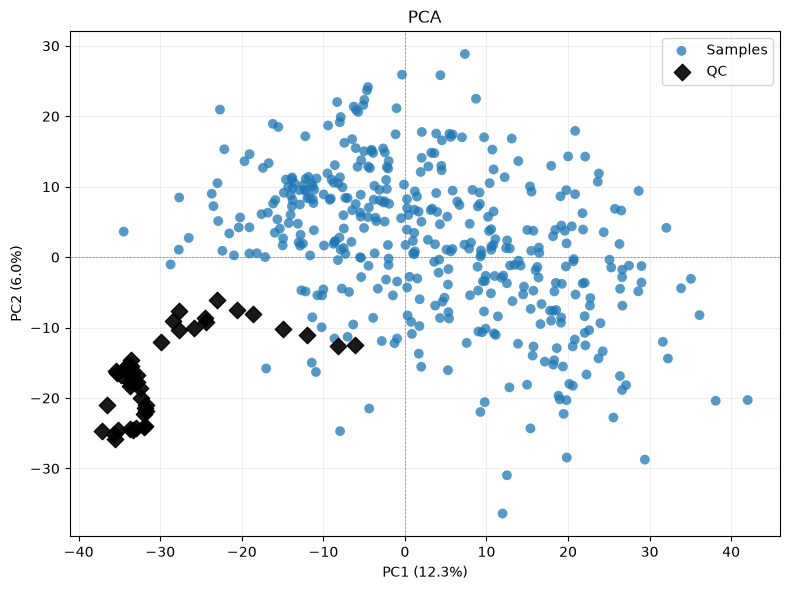
We see some clear indication of instrumental drift in the QC samples.
Run drift correction based on CPCA#
df_corrected = dc.run_cpca_drift_correction(df, sample_cols, qc_cols, n_comps=1)
Let’s plot the corrected data.
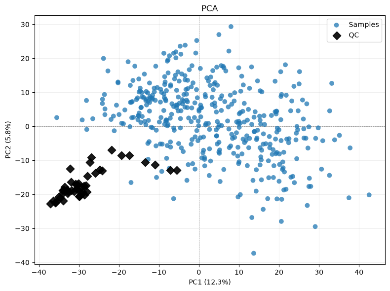
There is some change, but still a significant amount of drift is clearly visible from the PCA plot.
We can play around with the n_comps variable which decides the number of components.
df_corrected_2comps = dc.run_cpca_drift_correction(df, sample_cols, qc_cols, n_comps=2)
df_corrected_3comps = dc.run_cpca_drift_correction(df, sample_cols, qc_cols, n_comps=3)
df_corrected_4comps = dc.run_cpca_drift_correction(df, sample_cols, qc_cols, n_comps=4)
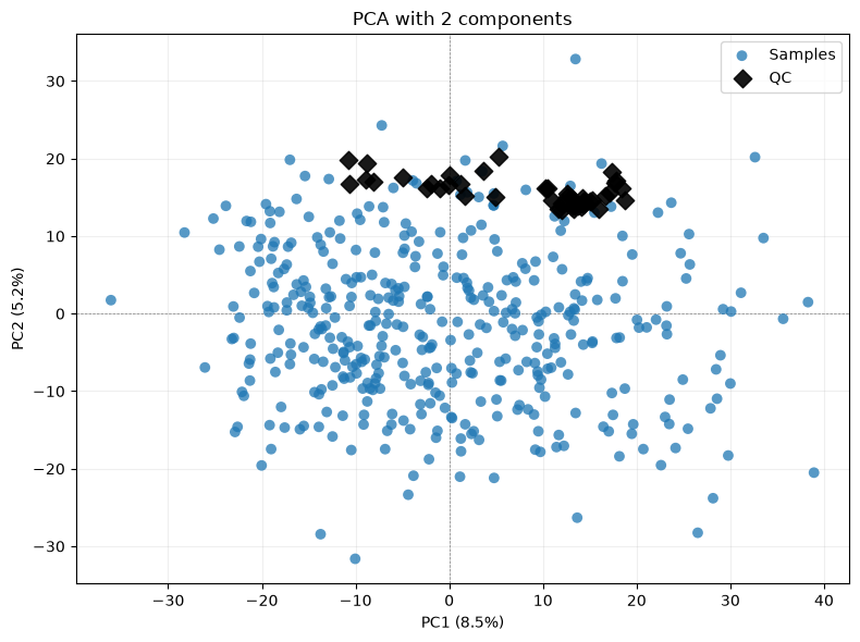
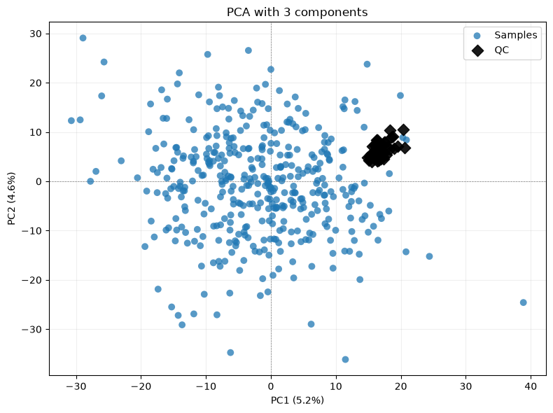
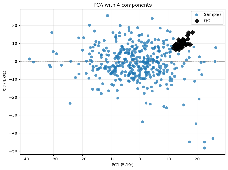
The correction methods with three and four components are already looking better. Let’s calculate the centroids of the QC principal components and the distance of the QC points to them, to objectively decide which number of n_comps is most favourable.
1 component: 6.659766536928962
2 components: 7.944509914596684
3 components: 1.8490307919985336
4 components: 2.251247334153261
According to this, the CPCA method with three principal components is most favourable in this case.
We can go ahead and continue our metabolomics data analysis with this data set.
df_corrected_3comps
| 0 | 1 | 2 | 3 | 4 | 5 | 6 | 7 | 8 | 9 | ... | 2,534 | 2,535 | 2,536 | 2,537 | 2,538 | 2,539 | 2,540 | 2,541 | 2,542 | 2,544 | |
|---|---|---|---|---|---|---|---|---|---|---|---|---|---|---|---|---|---|---|---|---|---|
| AAA9485207 | 264,911.666 | 76,093.970 | 107,731.115 | 41,789.199 | 17,777.028 | 208,108.097 | 306,494.837 | 121,963.335 | 44,889.022 | 49,012.511 | ... | 95,143.209 | 87,028.159 | 59,980.735 | 59,075.948 | 244,828.998 | 6,538,534.271 | 146,855.952 | 134,939.174 | 478,100.706 | 832,092.608 |
| AAA9485216 | 244,329.882 | 86,310.281 | 132,094.291 | 82,321.150 | 24,351.410 | 10,278.931 | 382,619.571 | 87,171.869 | 78,372.927 | 43,883.784 | ... | 138,195.868 | 125,428.392 | 84,809.253 | 68,058.862 | 228,344.182 | 4,676,645.012 | 53,646.032 | 127,037.161 | 496,962.146 | 1,182,481.025 |
| AAA9485239 | 121,545.312 | 87,838.557 | 148,081.789 | 72,700.333 | 33,388.147 | 10,176.755 | 428,086.054 | 186,668.522 | 76,799.608 | 43,731.288 | ... | 108,797.014 | 102,530.257 | 65,371.343 | 50,698.038 | 317,636.660 | 2,791,937.465 | 80,948.821 | 159,806.602 | 513,172.856 | 1,079,841.838 |
| AAA9485258 | 162,138.286 | 63,197.573 | 106,017.203 | 48,916.587 | 17,646.600 | 264,734.544 | 359,824.836 | 247,385.677 | 54,000.715 | 59,581.508 | ... | 150,801.967 | 131,711.745 | 103,686.397 | 76,351.244 | 240,164.597 | 3,511,612.142 | 114,593.775 | 95,345.264 | 275,433.247 | 690,675.171 |
| AAA9485261 | 161,038.603 | 68,937.047 | 118,463.154 | 61,758.290 | 20,026.160 | 226,478.584 | 292,481.564 | 194,665.402 | 54,494.756 | 42,554.703 | ... | 154,991.514 | 126,925.426 | 77,300.806 | 70,024.454 | 293,116.590 | 1,763,808.493 | 109,215.502 | 122,164.522 | 405,338.743 | 992,331.026 |
| ... | ... | ... | ... | ... | ... | ... | ... | ... | ... | ... | ... | ... | ... | ... | ... | ... | ... | ... | ... | ... | ... |
| QC_40 | 318,993.906 | 84,522.111 | 135,945.215 | 50,231.349 | 27,755.257 | 259,134.175 | 430,467.546 | 166,026.895 | 89,925.519 | 53,489.470 | ... | 137,906.342 | 121,833.542 | 97,626.237 | 76,460.554 | 223,249.699 | 5,587,889.118 | 117,029.993 | 175,457.154 | 513,082.085 | 939,820.835 |
| QC_41 | 322,126.443 | 70,822.062 | 138,438.511 | 66,830.331 | 34,336.715 | 263,851.296 | 430,584.410 | 154,843.010 | 94,461.601 | 58,447.505 | ... | 116,465.481 | 111,050.115 | 133,386.967 | 80,658.278 | 248,372.252 | 5,344,841.278 | 107,022.501 | 191,280.421 | 539,560.564 | 1,017,289.233 |
| QC_42 | 301,912.641 | 80,115.299 | 124,387.851 | 61,294.845 | 20,564.553 | 273,038.093 | 426,918.447 | 153,391.745 | 95,031.357 | 51,128.663 | ... | 124,406.926 | 124,794.934 | 90,877.844 | 76,611.083 | 232,267.111 | 4,772,819.371 | 90,008.901 | 212,727.546 | 610,192.128 | 1,103,739.770 |
| QC_43 | 275,656.649 | 79,188.791 | 142,043.838 | 57,809.475 | 25,500.161 | 275,890.702 | 408,854.157 | 165,587.772 | 91,769.175 | 48,987.886 | ... | 120,654.097 | 114,891.805 | 95,548.660 | 85,149.221 | 212,780.727 | 4,580,556.612 | 120,231.160 | 202,758.257 | 539,008.118 | 981,474.638 |
| QC_44 | 215,208.092 | 84,404.918 | 133,753.800 | 58,451.701 | 21,621.256 | 269,530.945 | 429,753.474 | 164,126.860 | 89,812.751 | 46,879.939 | ... | 128,429.509 | 119,914.776 | 97,422.963 | 83,167.893 | 231,041.389 | 6,134,909.597 | 96,677.520 | 194,838.649 | 541,233.603 | 978,352.995 |
477 rows × 2287 columns