Alzheimer’s MS-based proteomics

Proteome Profiling in Cerebrospinal Fluid Reveals Novel Biomarkers of Alzheimer’s Disease

• PXD016278

• publication

• curated data version from omiclearn

• download Alzheimer.xlsx from repository and process using data/prepare_alzheimer_excel.py as provided by njab, see njab

import numpy as np
import pandas as pd

import acore
import acore.types

BASE = (
    "https://raw.githubusercontent.com/RasmussenLab/njab/"
    "HEAD/docs/tutorial/data/alzheimer/"
)
META: str = "meta.csv"  # clincial data
CLINIC_ML: str = "clinic_ml.csv"  # clinical data
OMICS: str = "proteome.csv"  # omics data
freq_cutoff: float = (
    0.7  # at least x percent of samples must have a value for a feature (here: protein group)
)
#
covariates: list[str] = [
    "age",
    "male",
    "collection_site",
]  # clinical covariates to add to omics data
group: str = "AD"
subject_col: str = "Sample ID"
factor_and_covars: list[str] = [group, *covariates]

# BASE = (
#     "https://raw.githubusercontent.com/Multiomics-Analytics-Group/acore/"
#     "HEAD/example_data/MTBLS13311/"
#     ""
# )
# CLINIC_ML: str = "MTBLS13411_meta_data.csv"  # clinical data
# OMICS: str = "MTBLS13411_processed_data.csv"  # omics data
# covariates: list[str] = []
# group: str = "Factor Value[Strain type]"
# subject_col: str | int = 0
# factor_and_covars: list[str] = [group, *covariates]

Data

Clinical data:

Show code cell source

Hide code cell source

clinic = pd.read_csv(f"{BASE}/{CLINIC_ML}", index_col=subject_col).convert_dtypes()
omics = pd.read_csv(f"{BASE}/{OMICS}", index_col=subject_col)
meta = pd.read_csv(f"{BASE}/{META}", index_col=subject_col).convert_dtypes()
clinic

	Kiel	Magdeburg	Sweden	male	age	AD
Sample ID
Sample_000	0	0	1	0	71	0
Sample_001	0	0	1	1	77	1
Sample_002	0	0	1	1	75	1
Sample_003	0	0	1	0	72	1
Sample_004	0	0	1	0	63	1
...	...	...	...	...	...	...
Sample_205	0	0	0	0	69	1
Sample_206	0	0	0	1	73	0
Sample_207	0	0	0	0	71	0
Sample_208	0	0	0	1	83	0
Sample_209	0	0	0	0	63	0

210 rows × 6 columns

the variables for the collection site are based on the _collection site column in the metadata, which is binary (AD vs non-AD). We will add it to the clinic data here as collection_site

clinic["collection_site"] = meta["_collection site"].astype("category")
meta

	_collection site	_age at CSF collection	_gender	_t-tau [ng/L]	_p-tau [ng/L]	_Abeta-42 [ng/L]	_Abeta-40 [ng/L]	_Abeta-42/Abeta-40 ratio	_primary biochemical AD classification	_clinical AD diagnosis	_MMSE score
Sample ID
Sample_000	Sweden	71	f	703	85	562	<NA>	<NA>	biochemical control	<NA>	<NA>
Sample_001	Sweden	77	m	518	91	334	<NA>	<NA>	biochemical AD	<NA>	<NA>
Sample_002	Sweden	75	m	974	87	515	<NA>	<NA>	biochemical AD	<NA>	<NA>
Sample_003	Sweden	72	f	950	109	394	<NA>	<NA>	biochemical AD	<NA>	<NA>
Sample_004	Sweden	63	f	873	88	234	<NA>	<NA>	biochemical AD	<NA>	<NA>
...	...	...	...	...	...	...	...	...	...	...	...
Sample_205	Berlin	69	f	1945	<NA>	699	12140	0.058	biochemical AD	AD	17
Sample_206	Berlin	73	m	299	<NA>	1420	16571	0.086	biochemical control	non-AD	28
Sample_207	Berlin	71	f	262	<NA>	639	9663	0.066	biochemical control	non-AD	28
Sample_208	Berlin	83	m	289	<NA>	1436	11285	0.127	biochemical control	non-AD	24
Sample_209	Berlin	63	f	591	<NA>	1299	11232	0.116	biochemical control	non-AD	29

210 rows × 11 columns

Proteomics data:

Show code cell source

Hide code cell source

omics

	A0A024QZX5;A0A087X1N8;P35237	A0A024R0T9;K7ER74;P02655	A0A024R3B9;E9PJL7;E9PNH7;E9PR44;E9PRA8;P02511	A0A024R3W6;A0A024R412;O60462;O60462-2;O60462-3;O60462-4;O60462-5;Q7LBX6;X5D2Q8	A0A024R644;A0A0A0MRU5;A0A1B0GWI2;O75503	A0A075B6H7	A0A075B6H9	A0A075B6I0	A0A075B6I1	A0A075B6I6	...	Q9Y653;Q9Y653-2;Q9Y653-3	Q9Y696	Q9Y6C2	Q9Y6N6	Q9Y6N7;Q9Y6N7-2;Q9Y6N7-4	Q9Y6R7	Q9Y6X5	Q9Y6Y8;Q9Y6Y8-2	Q9Y6Y9	S4R3U6
Sample ID
Sample_000	61,673.895	118,287.297	NaN	48,660.887	91,474.398	161,523.438	1,243,916.125	111,328.523	196,418.406	129,966.305	...	66,103.219	37,065.340	NaN	33,928.590	117,492.836	953,704.750	NaN	774,452.625	7,319.069	7,157.334
Sample_001	62,683.871	120,084.656	NaN	46,952.789	85,696.211	14,219.552	1,006,628.062	452,086.125	144,818.047	NaN	...	47,247.086	48,831.750	NaN	29,184.250	99,154.422	1,290,353.000	48,161.156	685,002.875	16,046.540	5,566.107
Sample_002	70,801.492	23,540.432	NaN	62,662.648	87,425.625	295,910.656	623,874.625	116,678.055	52,162.660	132,150.766	...	38,397.008	27,131.826	13,840.273	35,567.586	177,753.438	793,489.750	54,547.285	1,429,741.250	6,367.055	5,811.354
Sample_003	70,579.844	133,966.578	NaN	57,126.406	129,144.039	63,886.270	810,226.938	236,600.234	481,605.812	18,580.904	...	46,175.461	24,667.812	26,278.039	36,111.652	167,765.281	705,753.312	NaN	1,217,899.750	6,326.341	5,574.454
Sample_004	49,777.762	41,204.301	NaN	42,501.414	104,929.156	45,487.113	1,432,224.125	420,529.000	138,671.141	18,056.232	...	27,682.402	34,978.043	16,933.244	39,127.047	138,061.406	784,805.750	41,140.680	956,304.688	9,055.216	4,819.975
...	...	...	...	...	...	...	...	...	...	...	...	...	...	...	...	...	...	...	...	...	...
Sample_205	52,580.969	121,142.914	17,094.783	30,787.574	91,553.039	NaN	213,644.766	134,705.750	NaN	87,260.188	...	38,577.703	52,639.848	19,290.646	43,690.750	192,023.203	248,320.922	82,961.828	997,297.812	7,800.822	3,571.952
Sample_206	56,974.930	192,433.844	39,391.934	49,655.160	62,771.391	NaN	291,774.688	291,227.625	92,853.867	118,952.797	...	43,910.461	70,548.422	NaN	41,630.660	138,975.266	428,263.688	19,466.387	707,613.188	NaN	NaN
Sample_207	54,708.844	120,377.539	NaN	45,354.527	122,102.547	NaN	407,462.125	253,284.094	81,851.984	86,517.844	...	57,367.875	70,132.867	21,659.680	53,800.195	98,345.039	433,233.062	72,127.773	794,190.062	12,739.789	2,310.061
Sample_208	45,602.434	112,493.625	NaN	32,653.695	71,837.844	NaN	30,733.824	189,291.719	NaN	71,154.883	...	36,545.277	107,334.961	NaN	25,528.732	94,810.352	697,161.188	57,325.840	764,947.125	9,514.913	NaN
Sample_209	54,229.551	157,105.312	41,592.316	36,990.523	77,132.398	NaN	243,478.969	219,587.188	84,727.141	56,250.707	...	38,610.566	51,480.586	37,939.453	18,884.396	110,151.523	634,252.562	54,416.516	782,212.562	2,108.535	3,544.341

210 rows × 1542 columns

Filtering data

If data is already filtered and/or imputed, skip this step.

Show code cell source

Hide code cell source

M_before = omics.shape[1]
omics = omics.dropna(thresh=int(len(omics) * freq_cutoff), axis=1)
M_after = omics.shape[1]
msg = (
    f"Removed {M_before-M_after} features "
    f"with more than {(1-freq_cutoff)*100:.2f}% missing values."
    f"\nRemaining features: {M_after} (of {M_before})"
)
print(msg)
# keep a map of all proteins in protein group, but only display first protein
# proteins are unique to protein groups
pg_map = {k: k.split(";")[0] for k in omics.columns}
omics = omics.rename(columns=pg_map)
# log2 transform raw intensity data:
omics = np.log2(omics + 1)
omics

Removed 432 features with more than 30.00% missing values.
Remaining features: 1110 (of 1542)

	A0A024QZX5	A0A024R0T9	A0A024R3W6	A0A024R644	A0A075B6H9	A0A075B6I0	A0A075B6I1	A0A075B6I6	A0A075B6I9	A0A075B6J9	...	Q9Y5Y7	Q9Y617	Q9Y646	Q9Y653	Q9Y696	Q9Y6N6	Q9Y6N7	Q9Y6R7	Q9Y6X5	Q9Y6Y8
Sample ID
Sample_000	15.912	16.852	15.571	16.481	20.246	16.764	17.584	16.988	20.054	NaN	...	18.840	16.859	19.322	16.012	15.178	15.050	16.842	19.863	NaN	19.563
Sample_001	15.936	16.874	15.519	16.387	19.941	18.786	17.144	NaN	19.067	16.188	...	19.195	16.799	19.190	15.528	15.576	14.833	16.597	20.299	15.556	19.386
Sample_002	16.112	14.523	15.935	16.416	19.251	16.832	15.671	17.012	18.569	NaN	...	19.088	16.288	19.702	15.229	14.728	15.118	17.440	19.598	15.735	20.447
Sample_003	16.107	17.032	15.802	16.979	19.628	17.852	18.877	14.182	18.985	13.438	...	18.715	17.075	19.760	15.495	14.590	15.140	17.356	19.429	NaN	20.216
Sample_004	15.603	15.331	15.375	16.679	20.450	18.682	17.081	14.140	19.686	14.495	...	18.668	16.736	19.624	14.757	15.094	15.256	17.075	19.582	15.328	19.867
...	...	...	...	...	...	...	...	...	...	...	...	...	...	...	...	...	...	...	...	...	...
Sample_205	15.682	16.886	14.910	16.482	17.705	17.039	NaN	16.413	19.102	16.064	...	18.726	15.808	19.894	15.236	15.684	15.415	17.551	17.922	16.340	19.928
Sample_206	15.798	17.554	15.600	15.938	18.155	18.152	16.503	16.860	18.538	15.288	...	18.460	15.035	20.015	15.422	16.106	15.345	17.084	18.708	14.249	19.433
Sample_207	15.740	16.877	15.469	16.898	18.636	17.950	16.321	16.401	18.849	17.580	...	19.502	16.283	20.306	15.808	16.098	15.715	16.586	18.725	16.138	19.599
Sample_208	15.477	16.779	14.995	16.132	14.908	17.530	NaN	16.119	18.368	15.202	...	18.892	15.920	20.203	15.157	16.712	14.640	16.533	19.411	15.807	19.545
Sample_209	15.727	17.261	15.175	16.235	17.893	17.744	16.371	15.780	18.806	16.532	...	18.675	15.713	20.042	15.237	15.652	14.205	16.749	19.275	15.732	19.577

210 rows × 1110 columns

Check if all values are numeric as this is required for differential analysis

acore.types.check_numeric_dataframe(omics)

	A0A024QZX5	A0A024R0T9	A0A024R3W6	A0A024R644	A0A075B6H9	A0A075B6I0	A0A075B6I1	A0A075B6I6	A0A075B6I9	A0A075B6J9	...	Q9Y5Y7	Q9Y617	Q9Y646	Q9Y653	Q9Y696	Q9Y6N6	Q9Y6N7	Q9Y6R7	Q9Y6X5	Q9Y6Y8
Sample ID
Sample_000	15.912	16.852	15.571	16.481	20.246	16.764	17.584	16.988	20.054	NaN	...	18.840	16.859	19.322	16.012	15.178	15.050	16.842	19.863	NaN	19.563
Sample_001	15.936	16.874	15.519	16.387	19.941	18.786	17.144	NaN	19.067	16.188	...	19.195	16.799	19.190	15.528	15.576	14.833	16.597	20.299	15.556	19.386
Sample_002	16.112	14.523	15.935	16.416	19.251	16.832	15.671	17.012	18.569	NaN	...	19.088	16.288	19.702	15.229	14.728	15.118	17.440	19.598	15.735	20.447
Sample_003	16.107	17.032	15.802	16.979	19.628	17.852	18.877	14.182	18.985	13.438	...	18.715	17.075	19.760	15.495	14.590	15.140	17.356	19.429	NaN	20.216
Sample_004	15.603	15.331	15.375	16.679	20.450	18.682	17.081	14.140	19.686	14.495	...	18.668	16.736	19.624	14.757	15.094	15.256	17.075	19.582	15.328	19.867
...	...	...	...	...	...	...	...	...	...	...	...	...	...	...	...	...	...	...	...	...	...
Sample_205	15.682	16.886	14.910	16.482	17.705	17.039	NaN	16.413	19.102	16.064	...	18.726	15.808	19.894	15.236	15.684	15.415	17.551	17.922	16.340	19.928
Sample_206	15.798	17.554	15.600	15.938	18.155	18.152	16.503	16.860	18.538	15.288	...	18.460	15.035	20.015	15.422	16.106	15.345	17.084	18.708	14.249	19.433
Sample_207	15.740	16.877	15.469	16.898	18.636	17.950	16.321	16.401	18.849	17.580	...	19.502	16.283	20.306	15.808	16.098	15.715	16.586	18.725	16.138	19.599
Sample_208	15.477	16.779	14.995	16.132	14.908	17.530	NaN	16.119	18.368	15.202	...	18.892	15.920	20.203	15.157	16.712	14.640	16.533	19.411	15.807	19.545
Sample_209	15.727	17.261	15.175	16.235	17.893	17.744	16.371	15.780	18.806	16.532	...	18.675	15.713	20.042	15.237	15.652	14.205	16.749	19.275	15.732	19.577

210 rows × 1110 columns

Validate the schema of the omics DataFrame. Builds and then uses the schema on the same data frame (experimental)

acore.types.build_schema_all_floats(omics).validate(omics)

	A0A024QZX5	A0A024R0T9	A0A024R3W6	A0A024R644	A0A075B6H9	A0A075B6I0	A0A075B6I1	A0A075B6I6	A0A075B6I9	A0A075B6J9	...	Q9Y5Y7	Q9Y617	Q9Y646	Q9Y653	Q9Y696	Q9Y6N6	Q9Y6N7	Q9Y6R7	Q9Y6X5	Q9Y6Y8
Sample ID
Sample_000	15.912	16.852	15.571	16.481	20.246	16.764	17.584	16.988	20.054	NaN	...	18.840	16.859	19.322	16.012	15.178	15.050	16.842	19.863	NaN	19.563
Sample_001	15.936	16.874	15.519	16.387	19.941	18.786	17.144	NaN	19.067	16.188	...	19.195	16.799	19.190	15.528	15.576	14.833	16.597	20.299	15.556	19.386
Sample_002	16.112	14.523	15.935	16.416	19.251	16.832	15.671	17.012	18.569	NaN	...	19.088	16.288	19.702	15.229	14.728	15.118	17.440	19.598	15.735	20.447
Sample_003	16.107	17.032	15.802	16.979	19.628	17.852	18.877	14.182	18.985	13.438	...	18.715	17.075	19.760	15.495	14.590	15.140	17.356	19.429	NaN	20.216
Sample_004	15.603	15.331	15.375	16.679	20.450	18.682	17.081	14.140	19.686	14.495	...	18.668	16.736	19.624	14.757	15.094	15.256	17.075	19.582	15.328	19.867
...	...	...	...	...	...	...	...	...	...	...	...	...	...	...	...	...	...	...	...	...	...
Sample_205	15.682	16.886	14.910	16.482	17.705	17.039	NaN	16.413	19.102	16.064	...	18.726	15.808	19.894	15.236	15.684	15.415	17.551	17.922	16.340	19.928
Sample_206	15.798	17.554	15.600	15.938	18.155	18.152	16.503	16.860	18.538	15.288	...	18.460	15.035	20.015	15.422	16.106	15.345	17.084	18.708	14.249	19.433
Sample_207	15.740	16.877	15.469	16.898	18.636	17.950	16.321	16.401	18.849	17.580	...	19.502	16.283	20.306	15.808	16.098	15.715	16.586	18.725	16.138	19.599
Sample_208	15.477	16.779	14.995	16.132	14.908	17.530	NaN	16.119	18.368	15.202	...	18.892	15.920	20.203	15.157	16.712	14.640	16.533	19.411	15.807	19.545
Sample_209	15.727	17.261	15.175	16.235	17.893	17.744	16.371	15.780	18.806	16.532	...	18.675	15.713	20.042	15.237	15.652	14.205	16.749	19.275	15.732	19.577

210 rows × 1110 columns

For easier inspection we just sample 100 protein groups. Remove this step in a real analysis.

Show code cell source

Hide code cell source

omics = omics.sample(min(omics.shape[1], 100), axis=1, random_state=42)
omics

	Q6UX72	O14773	A0A0A0MQU6	P36222	P51693-2	P17174	Q9BWS9	A0A0B4J2D9	P00734	Q13433	...	A0A075B6K4	O15041	J3KNA1	A0A0C4DH33	P16870	G3V533	Q9Y5I4	P55283	A1L4H1	Q7Z4T9
Sample ID
Sample_000	16.047	18.412	16.381	20.948	18.658	20.232	15.500	15.408	19.870	14.999	...	16.149	14.013	20.549	14.269	20.468	18.448	17.187	17.422	15.542	19.331
Sample_001	14.457	17.869	16.196	21.083	18.446	19.776	14.760	NaN	20.338	14.374	...	16.127	13.916	15.854	14.379	19.902	17.723	17.447	17.097	15.734	18.980
Sample_002	15.631	17.662	16.071	21.206	18.967	20.066	NaN	15.362	19.814	15.121	...	15.387	13.903	17.576	13.675	19.619	17.006	17.410	17.752	15.824	19.326
Sample_003	16.204	18.437	16.356	20.729	18.798	20.195	15.300	NaN	20.078	14.798	...	16.565	14.526	18.173	NaN	20.170	17.212	17.545	17.483	15.515	18.953
Sample_004	15.968	18.577	16.001	21.068	18.422	20.485	16.054	NaN	19.786	15.097	...	16.418	14.933	15.440	NaN	19.987	17.624	17.297	17.172	15.334	18.651
...	...	...	...	...	...	...	...	...	...	...	...	...	...	...	...	...	...	...	...	...	...
Sample_205	15.262	18.046	16.358	21.321	18.580	19.838	14.942	14.204	20.530	14.518	...	15.350	13.572	13.482	NaN	19.984	15.269	17.104	16.952	15.705	18.844
Sample_206	NaN	16.573	16.099	20.663	19.191	18.388	16.026	15.503	21.106	NaN	...	16.582	9.748	14.372	15.567	19.396	16.976	17.109	18.056	15.282	18.686
Sample_207	15.463	17.991	16.062	20.770	19.050	19.361	15.551	NaN	20.477	13.842	...	15.768	13.241	13.931	15.092	19.923	16.669	16.938	17.248	14.874	19.146
Sample_208	15.786	17.216	15.929	20.938	18.216	19.183	15.176	14.104	20.483	13.929	...	17.560	14.442	NaN	14.267	19.831	16.258	17.155	16.353	15.471	16.853
Sample_209	15.691	NaN	15.914	20.366	19.308	19.534	15.653	13.784	21.183	13.923	...	16.338	13.628	NaN	13.051	19.427	14.848	16.776	16.597	14.699	18.087

210 rows × 100 columns

Consider replacing with the filter from the acore package!

Preparing metadata

add both relevant clinical information to the omics data

Show code cell source

Hide code cell source

clinic[factor_and_covars].describe()

	AD	age	male
count	210.000	197.000	210.000
mean	0.419	67.726	0.467
std	0.495	12.123	0.500
min	0.000	20.000	0.000
25%	0.000	63.000	0.000
50%	0.000	70.000	0.000
75%	1.000	74.000	1.000
max	1.000	88.000	1.000

Show code cell source

Hide code cell source

omics_and_clinic = clinic[factor_and_covars].dropna().join(omics)
omics_and_clinic

	AD	age	male	collection_site	Q6UX72	O14773	A0A0A0MQU6	P36222	P51693-2	P17174	...	A0A075B6K4	O15041	J3KNA1	A0A0C4DH33	P16870	G3V533	Q9Y5I4	P55283	A1L4H1	Q7Z4T9
Sample ID
Sample_000	0	71	0	Sweden	16.047	18.412	16.381	20.948	18.658	20.232	...	16.149	14.013	20.549	14.269	20.468	18.448	17.187	17.422	15.542	19.331
Sample_001	1	77	1	Sweden	14.457	17.869	16.196	21.083	18.446	19.776	...	16.127	13.916	15.854	14.379	19.902	17.723	17.447	17.097	15.734	18.980
Sample_002	1	75	1	Sweden	15.631	17.662	16.071	21.206	18.967	20.066	...	15.387	13.903	17.576	13.675	19.619	17.006	17.410	17.752	15.824	19.326
Sample_003	1	72	0	Sweden	16.204	18.437	16.356	20.729	18.798	20.195	...	16.565	14.526	18.173	NaN	20.170	17.212	17.545	17.483	15.515	18.953
Sample_004	1	63	0	Sweden	15.968	18.577	16.001	21.068	18.422	20.485	...	16.418	14.933	15.440	NaN	19.987	17.624	17.297	17.172	15.334	18.651
...	...	...	...	...	...	...	...	...	...	...	...	...	...	...	...	...	...	...	...	...	...
Sample_205	1	69	0	Berlin	15.262	18.046	16.358	21.321	18.580	19.838	...	15.350	13.572	13.482	NaN	19.984	15.269	17.104	16.952	15.705	18.844
Sample_206	0	73	1	Berlin	NaN	16.573	16.099	20.663	19.191	18.388	...	16.582	9.748	14.372	15.567	19.396	16.976	17.109	18.056	15.282	18.686
Sample_207	0	71	0	Berlin	15.463	17.991	16.062	20.770	19.050	19.361	...	15.768	13.241	13.931	15.092	19.923	16.669	16.938	17.248	14.874	19.146
Sample_208	0	83	1	Berlin	15.786	17.216	15.929	20.938	18.216	19.183	...	17.560	14.442	NaN	14.267	19.831	16.258	17.155	16.353	15.471	16.853
Sample_209	0	63	0	Berlin	15.691	NaN	15.914	20.366	19.308	19.534	...	16.338	13.628	NaN	13.051	19.427	14.848	16.776	16.597	14.699	18.087

197 rows × 104 columns

Check that the added clinical metadata is numeric

• collection_site is a string

acore.types.check_numeric_dataframe(omics_and_clinic.drop(columns="collection_site"))

	AD	age	male	Q6UX72	O14773	A0A0A0MQU6	P36222	P51693-2	P17174	Q9BWS9	...	A0A075B6K4	O15041	J3KNA1	A0A0C4DH33	P16870	G3V533	Q9Y5I4	P55283	A1L4H1	Q7Z4T9
Sample ID
Sample_000	0	71	0	16.047	18.412	16.381	20.948	18.658	20.232	15.500	...	16.149	14.013	20.549	14.269	20.468	18.448	17.187	17.422	15.542	19.331
Sample_001	1	77	1	14.457	17.869	16.196	21.083	18.446	19.776	14.760	...	16.127	13.916	15.854	14.379	19.902	17.723	17.447	17.097	15.734	18.980
Sample_002	1	75	1	15.631	17.662	16.071	21.206	18.967	20.066	NaN	...	15.387	13.903	17.576	13.675	19.619	17.006	17.410	17.752	15.824	19.326
Sample_003	1	72	0	16.204	18.437	16.356	20.729	18.798	20.195	15.300	...	16.565	14.526	18.173	NaN	20.170	17.212	17.545	17.483	15.515	18.953
Sample_004	1	63	0	15.968	18.577	16.001	21.068	18.422	20.485	16.054	...	16.418	14.933	15.440	NaN	19.987	17.624	17.297	17.172	15.334	18.651
...	...	...	...	...	...	...	...	...	...	...	...	...	...	...	...	...	...	...	...	...	...
Sample_205	1	69	0	15.262	18.046	16.358	21.321	18.580	19.838	14.942	...	15.350	13.572	13.482	NaN	19.984	15.269	17.104	16.952	15.705	18.844
Sample_206	0	73	1	NaN	16.573	16.099	20.663	19.191	18.388	16.026	...	16.582	9.748	14.372	15.567	19.396	16.976	17.109	18.056	15.282	18.686
Sample_207	0	71	0	15.463	17.991	16.062	20.770	19.050	19.361	15.551	...	15.768	13.241	13.931	15.092	19.923	16.669	16.938	17.248	14.874	19.146
Sample_208	0	83	1	15.786	17.216	15.929	20.938	18.216	19.183	15.176	...	17.560	14.442	NaN	14.267	19.831	16.258	17.155	16.353	15.471	16.853
Sample_209	0	63	0	15.691	NaN	15.914	20.366	19.308	19.534	15.653	...	16.338	13.628	NaN	13.051	19.427	14.848	16.776	16.597	14.699	18.087

197 rows × 103 columns

Checking missing data

… between two AD groups (after previous filtering)

Show code cell source

Hide code cell source

data_completeness = (
    omics_and_clinic.groupby(by=group)
    .count()
    .divide(clinic[group].value_counts(), axis=0)
)
data_completeness

	age	male	collection_site	Q6UX72	O14773	A0A0A0MQU6	P36222	P51693-2	P17174	Q9BWS9	...	A0A075B6K4	O15041	J3KNA1	A0A0C4DH33	P16870	G3V533	Q9Y5I4	P55283	A1L4H1	Q7Z4T9
AD
0	0.893	0.893	0.893	0.869	0.844	0.844	0.893	0.893	0.893	0.689	...	0.861	0.607	0.656	0.770	0.893	0.877	0.885	0.893	0.828	0.861
1	1.000	1.000	1.000	1.000	0.966	0.977	1.000	1.000	1.000	0.705	...	0.932	0.830	0.705	0.693	1.000	0.989	0.989	1.000	0.966	0.989

2 rows × 103 columns

Plot number of missing values per group, ordered by proportion of non-misisng values in non-Alzheimer disease group

Show code cell source

Hide code cell source

sort_by = data_completeness.index[0]
ax = data_completeness.T.sort_values(sort_by).plot(
    style=".", ylim=(0, 1.05), alpha=0.5, rot=45
)

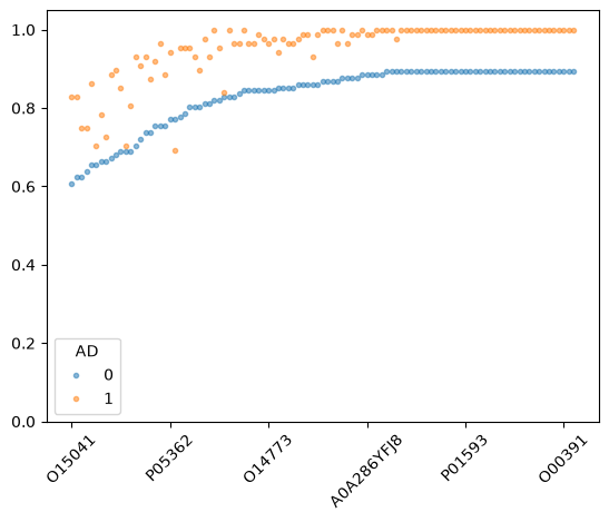
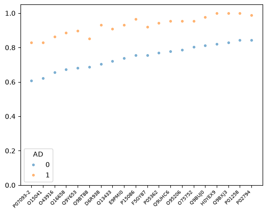
Plot 20 protein groups with biggest difference in missing values between groups

Show code cell source

Hide code cell source

idx_largerst_diff = (
    data_completeness.diff().dropna().T.squeeze().abs().nlargest(20).index
)
ax = (
    data_completeness.loc[:, idx_largerst_diff]
    .T.sort_values(sort_by)
    .plot(
        style=".",
        ylim=(0, 1.05),
        alpha=0.5,
        rot=45,
    )
)
_ = ax.set_xticks(range(len(idx_largerst_diff)))
_ = ax.set_xticklabels(
    idx_largerst_diff,
    rotation=45,
    ha="right",
    fontsize=7,
)

Save data for use in ANCOVA and ANOVA examples

omics_and_clinic.to_csv(
    "../../example_data/alzheimer_proteomics/alzheimer_example_omics_and_clinic.csv"
)

Done.