

Enrichment analysis#
requires
some cluster of proteins/genes (e.g. up- and downregulated proteins/genes)
functional annotations, i.e. a category summarizing a set of proteins/genes.
You can start with watching Lars Juhl Jensen’s brief introduction to enrichment analysis on youtube.
Here we use as example data from an ovarian cancer dataset: PXD010372
First make sure you have the required packages installed:
# ToDo: Improve VueCore dependencies
%pip install acore vuecore python-louvain snfpy
from pathlib import Path
import dsp_pandas
import pandas as pd
import acore
import acore.differential_regulation
import acore.enrichment_analysis
dsp_pandas.format.set_pandas_options(max_colwidth=60)
Parameters of this notebook
base_path: str = (
"https://raw.githubusercontent.com/Multiomics-Analytics-Group/acore/refs/heads/main/"
"example_data/PXD010372/processed"
)
omics: str = f"{base_path}/omics.csv"
meta_pgs: str = f"{base_path}/meta_pgs.csv"
meta: str = f"{base_path}/meta_patients.csv"
features_to_sample: int = 100
Load processed data#
from our repository. See details on obtaining the data under the example data section on this page
df_omics = pd.read_csv(omics, index_col=0)
df_meta_pgs = pd.read_csv(meta_pgs, index_col=0)
df_meta = pd.read_csv(meta, index_col=0)
df_omics
| P04217 | Q9NQ94-6 | P01023 | A8K2U0 | Q9NPC4 | Q9NRG9 | Q86V21 | Q7RTV5 | Q6PD74 | A0A096LP25 | ... | P06889 | P07951-2 | P09493-3 | P09493-8 | P0DMW5 | P23083 | P80748 | Q29967 | Q5T8P6-2 | Q5T8P6-3 | |
|---|---|---|---|---|---|---|---|---|---|---|---|---|---|---|---|---|---|---|---|---|---|
| Patient02 | 31.692 | 28.418 | 33.330 | 24.592 | 24.250 | 29.019 | 29.245 | NaN | 26.173 | 28.495 | ... | 25.704 | 32.095 | 30.611 | NaN | NaN | 25.947 | 27.607 | 28.401 | 24.711 | 28.975 |
| Patient24 | 32.113 | 27.401 | 33.009 | 25.149 | 24.902 | 29.400 | 28.924 | NaN | 24.706 | 27.410 | ... | 24.301 | 33.191 | 30.633 | 30.067 | NaN | 29.286 | 27.957 | 27.551 | 24.391 | 29.047 |
| Patient08 | 31.097 | 28.432 | 31.600 | 25.151 | NaN | 29.252 | 26.575 | NaN | NaN | 28.213 | ... | 23.590 | 32.968 | 31.439 | 28.936 | NaN | 28.306 | 29.456 | 29.775 | 25.486 | 28.924 |
| Patient03 | 30.995 | 28.365 | 33.827 | 22.606 | 23.793 | 29.446 | 29.296 | NaN | 24.301 | 28.854 | ... | NaN | 32.578 | 31.484 | 27.719 | NaN | 26.100 | 28.598 | 27.193 | NaN | 30.021 |
| Patient13 | 32.037 | NaN | 33.761 | 23.823 | NaN | 28.945 | 27.177 | NaN | 24.637 | 28.921 | ... | NaN | 34.461 | 32.920 | 28.884 | NaN | 29.893 | 31.016 | 29.931 | NaN | 29.517 |
| Patient18 | 31.855 | NaN | 34.705 | 25.289 | 25.377 | 27.779 | 26.758 | NaN | 24.226 | 27.896 | ... | 24.383 | 33.344 | 31.891 | 27.841 | NaN | 29.193 | 28.310 | 30.401 | NaN | 27.910 |
| Patient25 | 30.773 | NaN | 32.751 | NaN | NaN | 28.813 | 28.589 | NaN | 24.396 | 28.315 | ... | NaN | 30.589 | 29.244 | 24.012 | NaN | 27.692 | 24.011 | 27.139 | 25.195 | 29.448 |
| Patient14 | 30.435 | 28.195 | 32.463 | NaN | NaN | 29.564 | 28.233 | NaN | 25.189 | 30.207 | ... | 23.700 | 33.071 | 31.503 | 26.714 | NaN | 28.491 | 28.122 | 30.373 | 26.393 | 29.849 |
| Patient05 | 30.219 | 26.704 | 32.468 | 22.564 | NaN | 28.719 | 29.265 | 23.019 | 25.624 | 29.525 | ... | NaN | 30.435 | 29.425 | 25.293 | NaN | 27.293 | 27.931 | 30.291 | 26.618 | 29.479 |
| Patient20 | 31.078 | NaN | 34.063 | 25.315 | 24.377 | 28.385 | 27.472 | NaN | 24.626 | 28.666 | ... | NaN | 32.109 | 30.750 | 26.679 | NaN | 25.503 | NaN | 29.367 | 24.658 | 28.802 |
| Patient21 | 30.912 | NaN | 33.287 | NaN | NaN | 29.188 | 28.756 | NaN | NaN | 28.396 | ... | NaN | 33.239 | 31.750 | 27.464 | NaN | 29.800 | 29.206 | 30.769 | NaN | 30.355 |
| Patient11 | 30.697 | 28.426 | 32.712 | 22.730 | 23.259 | 29.753 | 28.441 | NaN | 24.970 | 26.765 | ... | 23.929 | 32.397 | 30.945 | 27.180 | 19.654 | 25.578 | 27.736 | 26.040 | 25.767 | 30.056 |
| Patient23 | 31.175 | 28.184 | 32.586 | 24.601 | NaN | 29.202 | 28.150 | 22.956 | 24.361 | 28.326 | ... | NaN | 34.423 | 32.661 | 28.921 | NaN | 25.794 | 27.847 | 28.916 | 25.984 | 29.626 |
| Patient16 | 30.172 | 27.839 | 32.827 | 30.132 | NaN | 29.329 | 28.857 | NaN | 22.695 | 29.167 | ... | 23.819 | 32.130 | 31.584 | 26.226 | NaN | 26.428 | 27.499 | 25.790 | 24.300 | 29.740 |
| Patient07 | 30.991 | 27.558 | 32.742 | 21.468 | NaN | 28.534 | 25.345 | NaN | 24.528 | 28.065 | ... | NaN | 33.581 | 32.539 | 28.420 | NaN | 27.072 | 23.853 | 28.670 | 24.996 | 28.872 |
| Patient17 | 31.484 | 27.751 | 34.503 | 23.818 | NaN | 29.059 | 27.084 | NaN | 25.798 | 28.339 | ... | NaN | 32.383 | 31.135 | 26.782 | NaN | 25.634 | 27.485 | 29.994 | 25.876 | 29.284 |
| Patient04 | 31.410 | 28.070 | 33.947 | 23.039 | 24.354 | 29.062 | 28.640 | NaN | 26.040 | 28.909 | ... | NaN | 32.452 | 31.515 | 25.965 | 20.206 | 25.193 | 25.081 | 27.299 | 25.836 | 29.756 |
| Patient10 | 30.540 | 26.970 | 33.911 | 24.601 | NaN | 29.826 | 28.359 | NaN | 24.734 | 29.186 | ... | 25.039 | 33.270 | 31.977 | 28.255 | 20.992 | 25.832 | 28.539 | 27.989 | 25.638 | 29.984 |
| Patient12 | 31.881 | 27.155 | 33.990 | 23.756 | NaN | 28.367 | 27.276 | NaN | 24.930 | 28.589 | ... | 26.967 | 33.719 | 32.595 | 28.613 | NaN | 29.269 | 28.899 | 27.364 | 25.619 | 28.604 |
| Patient06 | 31.969 | NaN | 33.707 | 22.169 | 24.041 | 29.420 | 27.533 | NaN | NaN | 28.196 | ... | NaN | 33.199 | 31.595 | 26.842 | NaN | 27.593 | 29.836 | 30.685 | NaN | 29.132 |
| Patient09 | 30.657 | 27.128 | 34.230 | NaN | NaN | 29.205 | 27.669 | NaN | 25.924 | 28.201 | ... | NaN | 31.685 | 31.324 | 25.805 | NaN | 27.592 | 26.667 | 29.753 | 25.349 | 28.876 |
| Patient15 | 30.606 | NaN | 34.209 | NaN | NaN | 28.476 | 26.708 | NaN | NaN | 28.343 | ... | NaN | 32.300 | 30.295 | 27.085 | NaN | 28.329 | 26.651 | 29.954 | 24.755 | 29.945 |
| Patient22 | 30.311 | NaN | 33.014 | NaN | NaN | 30.312 | 28.655 | NaN | 26.169 | 28.945 | ... | NaN | 33.099 | 31.663 | 28.124 | NaN | 26.345 | 26.829 | 31.376 | 25.959 | 30.301 |
| Patient19 | 30.641 | 28.844 | 32.556 | 21.944 | NaN | 28.835 | 27.235 | NaN | 23.146 | 29.000 | ... | 27.079 | 34.425 | 33.490 | 29.931 | NaN | 25.061 | 29.803 | 29.947 | 24.917 | 29.669 |
| Patient01 | 31.957 | 27.237 | 33.766 | NaN | NaN | 29.325 | 28.526 | NaN | 25.355 | 27.734 | ... | NaN | 33.243 | 31.817 | 28.737 | NaN | 26.888 | 28.780 | 29.021 | 24.186 | 29.075 |
25 rows × 8946 columns
ax = (
df_omics.notna()
.sum()
.sort_values(ascending=True)
.plot(xlabel="Protein groups", ylabel="Number of non-NaN values (samples)")
)
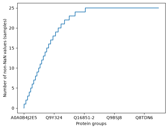
Keep only features with a certain amount of non-NaN values and select 100 of these for illustration. Add always four which were differently regulated in the ANOVA using all the protein groups.
idx_always_included = ["Q5HYN5", "P39059", "O43432", "O43175"]
| P62699 | Q9UID3 | P05186 | Q9NZ08-2 | Q8TF74 | O15230 | Q4LDE5 | Q96MG7 | Q96MM6 | Q9Y6M1 | ... | Q9UKU7 | Q96SY0 | Q13247 | Q9NQG5 | H3BPE1 | Q02833 | Q5HYN5 | P39059 | O43432 | O43175 | |
|---|---|---|---|---|---|---|---|---|---|---|---|---|---|---|---|---|---|---|---|---|---|
| Patient02 | 25.744 | 27.646 | 24.825 | 30.105 | 27.181 | 30.261 | 24.238 | 24.996 | 23.847 | 31.927 | ... | 27.326 | 28.245 | 32.740 | 30.372 | 31.685 | 27.180 | 21.868 | 27.572 | 28.485 | 33.119 |
| Patient24 | 24.782 | 28.443 | 29.958 | 30.665 | 27.706 | 31.103 | 24.776 | 25.533 | 26.667 | 33.517 | ... | 28.354 | 28.067 | 33.131 | 31.254 | 31.339 | 27.098 | 28.910 | 29.459 | 28.228 | 34.151 |
| Patient08 | 26.635 | 28.011 | 28.743 | 29.763 | 27.332 | 30.480 | 25.142 | 24.687 | 24.214 | 29.387 | ... | 29.053 | 28.057 | 33.009 | 30.139 | 32.116 | 27.397 | 22.516 | 29.585 | 28.366 | 33.274 |
| Patient03 | 26.761 | 28.331 | 31.520 | 30.090 | 28.091 | 31.936 | 23.985 | 26.385 | 25.443 | 32.362 | ... | 28.245 | 27.612 | 33.184 | 30.992 | 31.345 | 27.867 | 21.852 | 28.343 | 28.733 | 34.434 |
| Patient13 | 27.491 | 28.966 | 25.042 | 30.876 | 28.581 | 32.188 | 23.905 | NaN | 23.498 | 32.105 | ... | 29.292 | 27.442 | 32.153 | 30.045 | 33.332 | 27.116 | 22.424 | 28.045 | 27.983 | 34.268 |
| Patient18 | NaN | 28.413 | 26.452 | 31.216 | 26.199 | 31.185 | NaN | NaN | 25.005 | 29.415 | ... | 28.315 | 26.442 | 30.620 | 30.013 | 32.085 | 26.713 | 20.567 | 27.846 | 28.193 | 31.871 |
| Patient25 | 26.072 | 28.371 | 29.305 | 30.088 | 27.197 | 31.111 | NaN | 24.499 | 24.883 | 32.270 | ... | 30.104 | 28.211 | 32.010 | 30.054 | 31.429 | 27.101 | 32.377 | 26.086 | 29.177 | 32.313 |
| Patient14 | 25.697 | 28.411 | 29.425 | 30.873 | 28.360 | 30.412 | 24.295 | 25.174 | 24.068 | 29.663 | ... | 29.632 | 27.428 | 32.530 | 30.974 | 31.788 | 27.049 | 22.130 | 26.888 | 28.299 | 32.963 |
| Patient05 | 25.790 | 27.874 | 24.818 | 30.635 | 26.518 | 30.998 | 22.597 | 24.534 | 23.701 | 30.797 | ... | 30.055 | 27.575 | 32.700 | 31.005 | 32.052 | 27.766 | 20.647 | 26.527 | 28.401 | 34.023 |
| Patient20 | 24.959 | 28.080 | 28.632 | 31.084 | 27.257 | 31.072 | NaN | 26.595 | 26.129 | 30.246 | ... | 29.512 | 27.605 | 31.557 | 30.284 | 32.153 | 26.902 | 23.337 | 26.162 | 28.947 | 32.507 |
| Patient21 | 26.374 | 28.163 | 26.020 | 32.343 | 28.301 | 32.388 | NaN | 27.555 | 25.467 | 32.892 | ... | 27.160 | 28.573 | 32.214 | 30.846 | 33.233 | NaN | 26.163 | 29.583 | 29.314 | 35.208 |
| Patient11 | 26.322 | 28.512 | 24.235 | 30.513 | 27.941 | 29.219 | 22.882 | 25.260 | 24.900 | 31.671 | ... | 28.757 | 29.051 | 33.398 | 31.657 | 31.656 | 27.653 | 21.419 | 27.526 | 27.870 | 36.087 |
| Patient23 | 27.373 | 28.389 | 30.295 | 29.885 | 27.726 | 31.278 | 25.704 | 25.357 | 25.495 | 31.612 | ... | 28.840 | 26.112 | 32.362 | 30.252 | 33.521 | 27.126 | 34.031 | 25.931 | 28.749 | 32.247 |
| Patient16 | 26.506 | 28.278 | 25.537 | 31.184 | 27.227 | 31.622 | NaN | 25.053 | 23.493 | 30.575 | ... | 29.774 | 28.135 | 32.817 | 30.031 | 32.910 | 27.223 | 21.429 | 27.865 | 28.570 | 33.674 |
| Patient07 | 25.715 | 28.380 | 23.654 | 30.521 | 26.910 | 31.911 | 25.611 | 23.744 | 24.818 | 31.005 | ... | 29.628 | 27.409 | 32.266 | 31.832 | 31.961 | 26.905 | 22.464 | 27.488 | 28.138 | 33.236 |
| Patient17 | 25.473 | 28.345 | 30.136 | 30.880 | 26.721 | 31.207 | 24.561 | 24.923 | 25.746 | 32.288 | ... | 28.751 | 27.704 | 32.410 | 30.878 | 31.450 | 26.455 | 29.921 | 27.244 | 28.630 | 33.756 |
| Patient04 | 25.822 | 28.670 | 24.103 | 29.637 | 27.581 | 30.972 | 23.876 | 25.153 | 24.173 | 32.007 | ... | 30.339 | 28.168 | 32.742 | 32.067 | 32.545 | 26.369 | 22.766 | 27.709 | 28.948 | 35.473 |
| Patient10 | 25.030 | 28.168 | 26.021 | 28.449 | 27.842 | 30.552 | 23.629 | 25.732 | 23.999 | 30.608 | ... | 28.969 | 28.068 | 32.337 | 30.069 | 32.492 | 26.901 | 21.094 | 27.315 | 27.512 | 34.164 |
| Patient12 | 25.973 | 28.266 | 26.580 | 30.112 | 26.236 | 31.083 | 24.757 | 24.533 | 27.254 | 31.241 | ... | 27.793 | 27.567 | 31.930 | 30.296 | 31.856 | 26.808 | 31.242 | 26.390 | 28.174 | 33.836 |
| Patient06 | 25.617 | 28.657 | 26.296 | 31.600 | 27.061 | 32.144 | 23.811 | 25.055 | 23.839 | 32.003 | ... | 28.889 | 27.420 | 32.057 | 31.404 | 32.079 | 26.577 | NaN | 25.560 | 27.818 | 33.526 |
| Patient09 | 25.055 | 27.873 | 31.705 | 30.227 | 26.819 | 29.953 | 25.248 | 23.154 | 24.546 | 31.707 | ... | 29.256 | 28.608 | 32.115 | 31.012 | 32.551 | 26.535 | 22.485 | 26.217 | 28.025 | 33.992 |
| Patient15 | 25.904 | 28.484 | 26.286 | 31.581 | 27.025 | 31.919 | NaN | 24.286 | 25.358 | 29.530 | ... | 29.986 | 26.993 | 32.577 | 30.992 | 31.949 | 25.985 | 26.292 | 27.203 | 27.812 | 32.633 |
| Patient22 | 27.152 | 28.855 | 27.813 | 30.987 | 25.051 | 31.263 | NaN | 25.648 | 25.047 | 31.950 | ... | 28.964 | 27.956 | 32.560 | 31.377 | 35.067 | 27.832 | 28.504 | 25.517 | 29.120 | 32.710 |
| Patient19 | 25.428 | 27.820 | 25.893 | 31.397 | 26.895 | 31.800 | 25.152 | 24.925 | 28.137 | 32.429 | ... | 28.720 | 26.959 | 32.432 | 30.829 | 31.956 | 27.395 | 26.936 | 26.108 | 29.104 | 32.940 |
| Patient01 | 26.674 | 27.999 | 29.158 | 31.028 | 28.454 | 31.230 | 24.325 | 25.249 | 23.878 | 29.512 | ... | 29.177 | 28.620 | 31.388 | 30.507 | 33.021 | 28.021 | 22.630 | 26.846 | 28.062 | 33.601 |
25 rows × 100 columns
And we have the following patient metadata, from which we will use the Status column as
our dependent variable and the PlatinumValue as a covariate.
df_meta
| PlatinumValue | Days to platinum resistance | Disease free days | Overall survival days | Status | Refractory | |
|---|---|---|---|---|---|---|
| Patient_id | ||||||
| Patient02 | Resistant | -54 | 114 | 241 | deceased | y |
| Patient24 | Sensitive | 2,584 | 2,754 | 2,903 | deceased | n |
| Patient08 | Resistant | 31 | 211 | 228 | deceased | n |
| Patient03 | Resistant | -22 | 114 | 1,489 | deceased | y |
| Patient13 | Sensitive | 382 | 573 | 1,479 | deceased | n |
| Patient18 | Sensitive | 971 | 1,133 | 1,716 | deceased | n |
| Patient25 | Sensitive | 3,100 | 3,229 | 3,229 | alive | n |
| Patient14 | Sensitive | 440 | 580 | 1,106 | deceased | n |
| Patient05 | Resistant | 18 | 161 | 363 | deceased | n |
| Patient20 | Sensitive | 1,111 | 1,296 | 3,046 | alive | n |
| Patient21 | Sensitive | 1,271 | 1,498 | 1,573 | deceased | n |
| Patient11 | Resistant | -37 | 391 | 567 | deceased | n |
| Patient23 | Sensitive | 2,478 | 2,603 | 2,603 | alive | n |
| Patient16 | Sensitive | 462 | 663 | 1,347 | deceased | n |
| Patient07 | Resistant | 20 | 210 | 345 | deceased | n |
| Patient17 | Sensitive | 864 | 1,008 | 1,528 | deceased | n |
| Patient04 | Resistant | 29 | 155 | 485 | deceased | n |
| Patient10 | Resistant | 104 | 366 | 922 | deceased | n |
| Patient12 | Sensitive | 366 | 552 | 973 | deceased | n |
| Patient06 | Resistant | 52 | 190 | 790 | deceased | n |
| Patient09 | Resistant | 134 | 335 | 1,118 | deceased | n |
| Patient15 | Sensitive | 397 | 588 | 1,078 | deceased | n |
| Patient22 | Sensitive | 1,665 | 1,804 | 1,804 | alive | n |
| Patient19 | Sensitive | 1,051 | 1,188 | 1,467 | alive | n |
| Patient01 | Resistant | 11 | 113 | 280 | deceased | y |
ANOVA: Compute up and downregulated genes#
These will be used to find enrichments in the set of both up and downregulated genes.
group = "Status"
diff_reg = acore.differential_regulation.run_anova(
df_omics.join(df_meta[[group]]),
drop_cols=[],
subject=None,
group=group,
)
diff_reg.describe(exclude=["float"])
| identifier | test | correction | rejected | group1 | group2 | Method | |
|---|---|---|---|---|---|---|---|
| count | 100 | 100 | 100 | 100 | 100 | 100 | 100 |
| unique | 100 | 1 | 1 | 2 | 1 | 1 | 1 |
| top | P62699 | t-Test | FDR correction BH | False | deceased | alive | Unpaired t-test |
| freq | 1 | 100 | 100 | 96 | 100 | 100 | 100 |
diff_reg["rejected"] = diff_reg["rejected"].astype(bool) # ! needs to be fixed in anova
diff_reg.query("rejected")
| identifier | T-Statistics | pvalue | mean(group1) | mean(group2) | std(group1) | std(group2) | log2FC | test | correction | padj | rejected | group1 | group2 | FC | -log10 pvalue | Method | |
|---|---|---|---|---|---|---|---|---|---|---|---|---|---|---|---|---|---|
| 32 | Q96JJ3 | -3.897 | 0.001 | 28.031 | 28.584 | 0.562 | 0.119 | -0.553 | t-Test | FDR correction BH | 0.018 | True | deceased | alive | 0.682 | 3.139 | Unpaired t-test |
| 97 | P39059 | 5.938 | 0.000 | 27.561 | 25.961 | 1.057 | 0.235 | 1.600 | t-Test | FDR correction BH | 0.000 | True | deceased | alive | 3.031 | 5.324 | Unpaired t-test |
| 98 | O43432 | -6.045 | 0.000 | 28.278 | 29.019 | 0.414 | 0.155 | -0.741 | t-Test | FDR correction BH | 0.001 | True | deceased | alive | 0.598 | 4.873 | Unpaired t-test |
| 99 | O43175 | 5.248 | 0.000 | 33.864 | 32.543 | 0.945 | 0.256 | 1.321 | t-Test | FDR correction BH | 0.001 | True | deceased | alive | 2.498 | 4.533 | Unpaired t-test |
Download functional annotations, here pathways, for the protein groups#
in our selection of the dataset.
from acore.io.uniprot import fetch_annotations, process_annotations
fname_annotations = f"downloaded/annotations_{features_to_sample}.csv"
fname = Path(fname_annotations)
try:
annotations = pd.read_csv(fname, index_col=0)
print(f"Loaded annotations from {fname}")
except FileNotFoundError:
print(f"Fetching annotations for {df_omics.columns.size} UniProt IDs.")
FIELDS = "go_p,go_c,go_f"
annotations = fetch_annotations(df_omics.columns, fields=FIELDS)
annotations = process_annotations(annotations, fields=FIELDS)
# cache the annotations
fname.parent.mkdir(exist_ok=True, parents=True)
annotations.to_csv(fname, index=True)
annotations
Fetching annotations for 100 UniProt IDs.
Fetched: 100 / 100
| identifier | source | annotation | |
|---|---|---|---|
| 0 | P62699 | Gene Ontology (biological process) | cell population proliferation [GO:0008283] |
| 1 | P62699 | Gene Ontology (cellular component) | centrosome [GO:0005813] |
| 2 | P62699 | Gene Ontology (molecular function) | metal ion binding [GO:0046872] |
| 3 | P62699 | Gene Ontology (cellular component) | extracellular region [GO:0005576] |
| 4 | P62699 | Gene Ontology (cellular component) | ficolin-1-rich granule lumen [GO:1904813] |
| ... | ... | ... | ... |
| 1,767 | O43175 | Gene Ontology (molecular function) | L-malate dehydrogenase (NAD+) activity [GO:0030060] |
| 1,768 | O43175 | Gene Ontology (molecular function) | NAD binding [GO:0051287] |
| 1,769 | O43175 | Gene Ontology (molecular function) | phosphoglycerate dehydrogenase activity [GO:0004617] |
| 1,770 | O43175 | Gene Ontology (cellular component) | extracellular exosome [GO:0070062] |
| 1,771 | O43175 | Gene Ontology (biological process) | L-serine biosynthetic process [GO:0006564] |
1752 rows × 3 columns
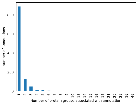
See how many protein groups are associated with each annotation. We observe that most functional annotations are associated only to a single protein group in our dataset.
| N protein groups | 1 | 2 | 3 | 4 | 5 | 6 | 7 | 8 | 9 | 10 | 13 | 14 | 15 | 16 | 18 | 21 | 25 | 28 | 36 | 46 |
|---|---|---|---|---|---|---|---|---|---|---|---|---|---|---|---|---|---|---|---|---|
| number of annotations | 887 | 130 | 48 | 13 | 8 | 6 | 4 | 2 | 2 | 1 | 1 | 2 | 2 | 1 | 1 | 1 | 1 | 1 | 1 | 1 |
annotations.groupby("annotation").size().value_counts(ascending=False)
1 887
2 130
3 48
4 13
5 8
6 6
7 4
8 2
15 2
14 2
9 2
28 1
18 1
21 1
10 1
36 1
46 1
16 1
25 1
13 1
Name: count, dtype: int64
Enrichment analysis#
Is done separately for up- and downregulated genes as it’s assumed that biological processes are regulated in one direction.
| identifier | group1 | group2 | pvalue | padj | rejected | log2FC | FC | |
|---|---|---|---|---|---|---|---|---|
| 98 | O43432 | deceased | alive | 0.000 | 0.001 | True | -0.741 | 0.598 |
| 32 | Q96JJ3 | deceased | alive | 0.001 | 0.018 | True | -0.553 | 0.682 |
| 99 | O43175 | deceased | alive | 0.000 | 0.001 | True | 1.321 | 2.498 |
| 97 | P39059 | deceased | alive | 0.000 | 0.000 | True | 1.600 | 3.031 |
Running the enrichment analysis for the up- and down regulated protein groups separately with the default settings of the function, i.e. a log2 fold change cutoff of 1 and at least 2 protein groups detected in the set of proteins defining the functional annotation.
ret = acore.enrichment_analysis.run_up_down_regulation_enrichment(
regulation_data=diff_reg,
annotation=annotations,
pval_col="padj",
min_detected_in_set=2,
lfc_cutoff=1,
)
No significant enrichment found with the given parameters. Returning an empty DataFrame.
we can decrease the cutoff for the log2 fold change to 0.5 and see that we retain more annotations.
ret = acore.enrichment_analysis.run_up_down_regulation_enrichment(
regulation_data=diff_reg,
annotation=annotations,
pval_col="padj",
min_detected_in_set=2,
lfc_cutoff=0.5, # ! the default is 1
)
No significant enrichment found with the given parameters. Returning an empty DataFrame.
And even more if we do not restrict the analysis of finding at least two proteins of a functional set in our data set (i.e. we only need to find one match from the set).
ret = acore.enrichment_analysis.run_up_down_regulation_enrichment(
regulation_data=diff_reg,
annotation=annotations,
pval_col="padj",
min_detected_in_set=1,
lfc_cutoff=0.5, # ! the default is 1
)
Site specific enrichment analysis#
The basic example uses a modified peptide sequence to demonstrate the enrichment analysis.
TODO: The example on how to do that needs a PTM focused dataset. The details of how site specific enrichment analysis is done will depend on the dataset and the question at hand.
If the identifiers contain PTMs this information is removed to match it to the annotation using a regular expression (in the function). For example:
import re
regex = "(\\w+~.+)_\\w\\d+\\-\\w+"
identifier_ckg = "gnd~P00350_T10-WW"
match = re.search(regex, identifier_ckg)
match.group(1)
'gnd~P00350'
# ToDo: Add example for site specific enrichment analysis
Single sample GSEA (ssGSEA)#
Run a gene set enrichment analysis (GSEA) for each sample. The ssGSEA is a method that the proteins (genes) are ordered for each sample and the ranking of proteins (genes) associated to a functional annotation (pathway, GO term, etc.) is used to compute an enrichment score for that sample for that functional annotation.
Method description accoring to Barbie et. al. (2009)
Note: The call functional annotation “signature” in the original article.
“This was accomplished by a ‘single sample’ extension of GSEA that allows one to define an enrichment score that represents the degree of absolute enrichment of a gene set in each sample within a given data set. The gene expression values for a given sample were rank-normalized, and an enrichment score was produced using the Empirical Cumulative Distribution Functions (ECDF) of the genes in the signature and the remaining genes. This procedure is similar to GSEA but the list is ranked by absolute expression (in one sample). The enrichment score is obtained by an integration of the difference between the ECDF. For a given signature \(G\) of size \(N_G\) and single sample \(S\), of the data set of \(N\) genes, the genes are replaced by their ranks according the their absolute expression: \(L=\{r_1, r_2, \ldots, r_N\}\). The list is then ordered from the highest rank \(N\) to the lowest \(1\). An enrichment score \(ES(G,S)\) is obtained by a sum (integration) of the difference between a weighted ECDF of the genes in the signature \(P_{G}^w\) and the ECDF of the remaining genes \(P_{NG}\):
\(ES(G,S) = \sum_{i=1}^{N} \left| P_{G}^{w}(G,S,i) - P_{N_G}(G,S,i) \right|\)
where
\(P_{G}^{w}(G,S,i)= \sum_{r_j \in G, j \leq i} \frac{|r_j|^\alpha}{\sum_{r_{j \in G}} |r_j|^\alpha}\) and \(P_{N_G}(G,S,i)= \sum_{r_j \notin G, j \leq i} \frac{1}{N - N_G}\)
This calculation is repeated for each signature and each sample in the data set. Note that the exponent of this quantity (\(α\)) is set to 1/4, and adds a modest weight to the rank. In the regular GSEA a similar enrichment score is used, but the weight is typically set to 1. Also, instead of the sum over \(i\), the enrichment score is computed according to the largest difference. This quantity is slightly more robust and more sensitive to differences in the tails of the distributions than the Kolmogorov–Smirnov statistic. It is particularly well suited to represent the activation score of gene sets on the basis of a relatively small subset of the genes attaining high expression values.” (Barbie et al., 2009)
See the above details from the
article and
the package
gseapy
for more details.
enrichtments = acore.enrichment_analysis.run_ssgsea(
data=df_omics,
annotation=annotations,
min_size=1,
)
enrichtments
2026-06-16 20:40:04,088 [WARNING] Input data contains NA, filled NA with 0
| Term | ES | NES | |
|---|---|---|---|
| Name | |||
| Patient22 | integrin binding [GO:0005178] | -50.000 | -0.500 |
| Patient24 | intracellular protein localization [GO:0008104] | -50.000 | -0.500 |
| Patient11 | electron transfer activity [GO:0009055] | 50.000 | 0.500 |
| Patient11 | brain development [GO:0007420] | 50.000 | 0.500 |
| Patient24 | positive regulation of cold-induced thermogenesis [GO:01... | -50.000 | -0.500 |
| ... | ... | ... | ... |
| Patient06 | focal adhesion [GO:0005925] | -0.054 | -0.001 |
| Patient01 | nervous system development [GO:0007399] | 0.052 | 0.001 |
| Patient23 | positive regulation of gene expression [GO:0010628] | -0.047 | -0.000 |
| Patient16 | RNA cap binding [GO:0000339] | 0.031 | 0.000 |
| Patient12 | cytoplasm [GO:0005737] | -0.010 | -0.000 |
4700 rows × 3 columns
enrichtments.iloc[0].to_dict()
{'Term': 'integrin binding [GO:0005178]', 'ES': -50.0, 'NES': -0.5}
ax = enrichtments["NES"].plot.hist()
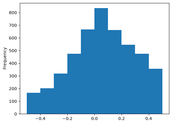
The normalised enrichment score (NES) can be used in a PCA plot to see if the samples cluster according to the enrichment of the gene sets.
nes = enrichtments.set_index("Term", append=True).unstack()["NES"].convert_dtypes()
nes
| Term | ATP binding [GO:0005524] | ATP hydrolysis activity [GO:0016887] | DNA repair [GO:0006281] | DNA-binding transcription factor binding [GO:0140297] | DNA-templated transcription [GO:0006351] | EKC/KEOPS complex [GO:0000408] | INTAC complex [GO:0160232] | LBD domain binding [GO:0050693] | NADP binding [GO:0050661] | P-body [GO:0000932] | ... | transcription coregulator activity [GO:0003712] | transcription corepressor activity [GO:0003714] | translation initiation factor activity [GO:0003743] | translational initiation [GO:0006413] | tubulin binding [GO:0015631] | ubiquitin ligase complex [GO:0000151] | ubiquitin protein ligase activity [GO:0061630] | ubiquitin protein ligase binding [GO:0031625] | visual perception [GO:0007601] | zinc ion binding [GO:0008270] |
|---|---|---|---|---|---|---|---|---|---|---|---|---|---|---|---|---|---|---|---|---|---|
| Name | |||||||||||||||||||||
| Patient01 | 0.057 | 0.364 | -0.086 | 0.146 | -0.095 | 0.207 | 0.025 | -0.035 | 0.409 | 0.146 | ... | -0.180 | -0.180 | -0.056 | -0.056 | 0.104 | -0.071 | -0.086 | 0.125 | -0.480 | 0.004 |
| Patient02 | 0.056 | 0.338 | 0.045 | 0.268 | -0.197 | 0.146 | -0.005 | -0.096 | 0.359 | 0.268 | ... | 0.118 | 0.118 | 0.015 | 0.015 | 0.129 | -0.071 | 0.045 | 0.166 | -0.480 | 0.104 |
| Patient03 | 0.040 | 0.325 | -0.298 | 0.177 | -0.207 | 0.116 | -0.136 | -0.187 | 0.227 | 0.177 | ... | 0.132 | 0.132 | 0.015 | 0.015 | 0.025 | -0.069 | -0.298 | 0.044 | -0.288 | -0.033 |
| Patient04 | -0.007 | 0.336 | -0.126 | 0.237 | 0.012 | 0.187 | -0.045 | -0.076 | 0.328 | 0.237 | ... | 0.081 | 0.081 | 0.066 | 0.066 | 0.064 | -0.040 | -0.126 | 0.118 | -0.177 | 0.015 |
| Patient05 | 0.021 | 0.347 | -0.025 | 0.237 | -0.042 | 0.116 | -0.136 | -0.035 | 0.399 | 0.237 | ... | -0.151 | -0.151 | 0.015 | 0.015 | 0.099 | -0.025 | -0.025 | 0.128 | -0.399 | 0.067 |
| Patient06 | 0.025 | 0.345 | -0.227 | 0.258 | -0.131 | 0.126 | -0.126 | -0.258 | 0.318 | 0.258 | ... | 0.004 | 0.004 | -0.066 | -0.066 | 0.088 | -0.134 | -0.227 | 0.095 | -0.419 | -0.061 |
| Patient07 | 0.019 | 0.363 | -0.258 | 0.227 | -0.030 | 0.217 | -0.126 | -0.146 | 0.359 | 0.227 | ... | -0.206 | -0.206 | -0.056 | -0.056 | 0.148 | -0.052 | -0.258 | 0.089 | -0.480 | -0.046 |
| Patient08 | 0.031 | 0.318 | -0.197 | 0.268 | -0.092 | 0.217 | -0.086 | -0.106 | 0.369 | 0.268 | ... | -0.117 | -0.117 | -0.066 | -0.066 | 0.026 | -0.076 | -0.197 | 0.067 | -0.490 | 0.035 |
| Patient09 | 0.038 | 0.347 | -0.045 | 0.157 | -0.070 | 0.146 | 0.045 | -0.066 | 0.419 | 0.157 | ... | -0.139 | -0.139 | -0.056 | -0.056 | 0.053 | -0.014 | -0.045 | 0.139 | -0.288 | 0.035 |
| Patient10 | 0.096 | 0.326 | -0.177 | 0.247 | -0.122 | 0.197 | -0.066 | -0.076 | 0.328 | 0.247 | ... | -0.051 | -0.051 | -0.126 | -0.126 | 0.128 | -0.019 | -0.177 | 0.083 | -0.348 | 0.006 |
| Patient11 | 0.063 | 0.366 | -0.177 | 0.278 | -0.110 | -0.066 | 0.106 | -0.045 | 0.318 | 0.278 | ... | -0.191 | -0.191 | -0.035 | -0.035 | 0.154 | -0.010 | -0.177 | 0.067 | -0.227 | 0.037 |
| Patient12 | 0.002 | 0.326 | 0.025 | 0.177 | -0.198 | 0.167 | -0.106 | -0.217 | 0.399 | 0.177 | ... | -0.035 | -0.035 | -0.035 | -0.035 | 0.102 | -0.116 | 0.025 | 0.133 | -0.419 | 0.090 |
| Patient13 | 0.024 | 0.329 | -0.409 | 0.136 | -0.120 | 0.086 | -0.157 | -0.227 | 0.328 | 0.136 | ... | 0.027 | 0.027 | -0.106 | -0.106 | 0.120 | -0.039 | -0.409 | 0.076 | -0.419 | -0.091 |
| Patient14 | 0.068 | 0.348 | -0.157 | 0.268 | -0.104 | 0.227 | -0.116 | -0.066 | 0.429 | 0.268 | ... | -0.195 | -0.195 | -0.045 | -0.045 | 0.083 | -0.019 | -0.157 | 0.068 | -0.278 | 0.015 |
| Patient15 | 0.097 | 0.367 | -0.066 | 0.298 | -0.043 | 0.258 | -0.177 | 0.005 | 0.268 | 0.298 | ... | -0.148 | -0.148 | -0.076 | -0.076 | 0.090 | 0.041 | -0.066 | 0.159 | -0.298 | 0.060 |
| Patient16 | 0.010 | 0.326 | -0.217 | 0.187 | -0.054 | 0.066 | -0.096 | -0.086 | 0.268 | 0.187 | ... | -0.097 | -0.097 | -0.025 | -0.025 | 0.082 | -0.040 | -0.217 | 0.066 | -0.258 | 0.012 |
| Patient17 | 0.030 | 0.313 | -0.167 | 0.197 | -0.145 | 0.136 | -0.096 | -0.207 | 0.369 | 0.197 | ... | 0.107 | 0.107 | -0.025 | -0.025 | 0.064 | -0.123 | -0.167 | 0.099 | -0.359 | 0.011 |
| Patient18 | 0.044 | 0.405 | -0.066 | 0.258 | 0.012 | 0.136 | -0.167 | -0.308 | 0.359 | 0.258 | ... | -0.346 | -0.346 | 0.045 | 0.045 | 0.128 | -0.153 | -0.066 | 0.124 | -0.439 | 0.072 |
| Patient19 | 0.007 | 0.338 | -0.106 | 0.187 | -0.156 | 0.167 | -0.207 | -0.348 | 0.389 | 0.187 | ... | 0.012 | 0.012 | 0.056 | 0.056 | 0.130 | -0.173 | -0.106 | 0.117 | -0.369 | 0.049 |
| Patient20 | 0.041 | 0.366 | -0.106 | 0.056 | 0.049 | 0.035 | -0.056 | -0.348 | 0.369 | 0.056 | ... | -0.403 | -0.403 | 0.076 | 0.076 | 0.038 | -0.198 | -0.106 | 0.110 | -0.449 | 0.024 |
| Patient21 | -0.011 | 0.351 | -0.439 | 0.278 | -0.232 | 0.126 | 0.005 | -0.217 | 0.318 | 0.278 | ... | 0.129 | 0.129 | 0.076 | 0.076 | 0.088 | -0.088 | -0.439 | 0.051 | -0.449 | -0.079 |
| Patient22 | 0.044 | 0.263 | -0.187 | 0.157 | -0.065 | 0.207 | -0.086 | -0.066 | 0.328 | 0.157 | ... | -0.019 | -0.019 | 0.066 | 0.066 | 0.091 | 0.013 | -0.187 | 0.096 | -0.268 | -0.011 |
| Patient23 | -0.023 | 0.331 | 0.066 | 0.247 | -0.050 | 0.167 | -0.278 | -0.136 | 0.278 | 0.247 | ... | -0.019 | -0.019 | 0.025 | 0.025 | 0.109 | -0.064 | 0.066 | 0.177 | -0.217 | 0.122 |
| Patient24 | 0.029 | 0.334 | -0.096 | 0.237 | -0.165 | 0.056 | -0.106 | -0.086 | 0.369 | 0.237 | ... | 0.157 | 0.157 | -0.066 | -0.066 | 0.080 | -0.082 | -0.096 | 0.104 | -0.449 | 0.043 |
| Patient25 | 0.100 | 0.330 | 0.015 | 0.116 | -0.040 | 0.298 | -0.086 | -0.146 | 0.318 | 0.116 | ... | -0.254 | -0.254 | 0.056 | 0.056 | 0.039 | -0.074 | 0.015 | 0.197 | -0.268 | 0.056 |
25 rows × 188 columns
import acore.exploratory_analysis as ea
pca_result, pca_annotation = ea.run_pca(
data=nes.join(df_meta[[group]]),
drop_cols=[],
annotation_cols=[],
group=group,
components=2,
dropna=False,
)
resultDf, loadings, var_exp = pca_result
resultDf
| group | x | y | |
|---|---|---|---|
| 0 | deceased | -1.336 | -0.011 |
| 1 | deceased | 1.077 | -0.587 |
| 2 | deceased | 1.403 | -0.276 |
| 3 | deceased | 0.755 | -0.022 |
| 4 | deceased | -0.785 | 0.561 |
| 5 | deceased | 0.804 | 0.468 |
| 6 | deceased | -0.760 | -0.215 |
| 7 | deceased | -0.294 | -0.724 |
| 8 | deceased | -0.632 | 0.506 |
| 9 | deceased | 0.053 | 0.427 |
| 10 | deceased | -1.127 | 0.297 |
| 11 | deceased | 0.557 | 0.050 |
| 12 | deceased | 0.932 | -0.174 |
| 13 | deceased | -1.143 | -0.457 |
| 14 | deceased | -1.122 | 0.693 |
| 15 | deceased | -0.194 | 0.345 |
| 16 | deceased | 1.257 | -0.209 |
| 17 | deceased | -1.244 | -0.798 |
| 18 | alive | 0.988 | -0.037 |
| 19 | alive | -1.506 | -0.197 |
| 20 | deceased | 1.548 | -0.364 |
| 21 | alive | 0.224 | 0.519 |
| 22 | alive | 0.433 | 0.108 |
| 23 | deceased | 1.407 | 0.493 |
| 24 | alive | -1.295 | -0.397 |
The loadings show how the variables are correlated with the principal components.
loadings
| x | y | value | |
|---|---|---|---|
| regulation of vesicle-mediated transport [GO:0060627] | 0.055 | 0.430 | 0.433 |
| protein transport [GO:0015031] | 0.055 | 0.430 | 0.433 |
| recycling endosome [GO:0055037] | 0.055 | 0.430 | 0.433 |
| endodermal cell differentiation [GO:0035987] | 0.296 | -0.020 | 0.297 |
| positive regulation of stem cell proliferation [GO:2000648] | 0.296 | -0.020 | 0.297 |
| ... | ... | ... | ... |
| scaffold protein binding [GO:0097110] | -0.006 | 0.000 | 0.006 |
| microtubule binding [GO:0008017] | -0.004 | -0.001 | 0.004 |
| catalytic step 2 spliceosome [GO:0071013] | -0.001 | 0.000 | 0.002 |
| spliceosomal complex [GO:0005681] | -0.001 | 0.000 | 0.002 |
| ribonucleoprotein complex [GO:1990904] | -0.001 | 0.000 | 0.002 |
188 rows × 3 columns
We will plot both on the sample plot (samples on the first two principal components and
loadings of variables). We use the
vuecore package
for this, which is also developed by the Multiomics Analytics Group.
import plotly.graph_objects as go
from vuecore import viz
args = {"factor": 2, "loadings": 1} # increase number of loadings or scaling factor
#! pca_results has three items, but docstring requests only two -> double check
figure = viz.get_pca_plot(data=pca_result, identifier="PCA enrichment", args=args)
figure = go.Figure(data=figure["data"], layout=figure["layout"])
figure
Compare two distributions - KS test#
The Kolmogorov-Smirnov test is a non-parametric test that compares two distributions.
we compare the distributions of the two differently upregulated protein groups This is not the best example for comparing distributions, but it shows how to use the KS test.
# plot two histograms of intensity values here
sel_pgs = ["O43175", "P39059"]
view = df_omics[sel_pgs].sub(df_omics[sel_pgs].mean())
ax = view.plot.hist(bins=20, alpha=0.5)
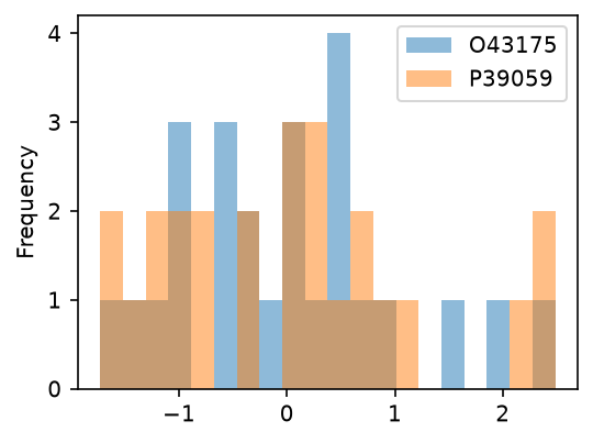
Let us compare the two centered distributions using the KS test.
acore.enrichment_analysis.run_kolmogorov_smirnov(view[sel_pgs[0]], view[sel_pgs[1]])
KstestResult(statistic=np.float64(0.12), pvalue=np.float64(0.995531553175167), statistic_location=np.float64(-1.0237811999999984), statistic_sign=np.int8(-1))
The result suggests that the two distributions are from the same distribution.
Done.