

Metabolomics data filtering#
This example notebook shows how to use the acore filtering functions specific for metabolomics data.
Scroll to read about the following methods:
80%-rule
modified 80%-rule
CV-based filtering
Blanks-based filtering
Apply whichever one fits your data best, or a combination of multiple. Adjust the thresholds to match your data and desired stringency.
%pip install acore
Data preparation#
Load in your data. The example data set can be found in
example_data/DidacMauricio_hilic.
data_path = (
    "https://raw.githubusercontent.com/Multiomics-Analytics-Group/acore/"
    "refs/heads/main/"
)
data_path = (
    "../../example_data/DidacMauricio_hilic/DM_FIS2018_Hilic_pos_results2023_filled.csv"
)
data_original = pd.read_csv(data_path)
We can now inspect our data:
| Qidx | SOIidx | rtmed | start | end | mass | MaxInt | formula | anot | AAA9485207 | ... | QC_35 | QC_36 | QC_37 | QC_38 | QC_39 | QC_40 | QC_41 | QC_42 | QC_43 | QC_44 | |
|---|---|---|---|---|---|---|---|---|---|---|---|---|---|---|---|---|---|---|---|---|---|
| 0 | 1 | 1 | 60.544 | 45.000 | 72.500 | 81.070 | 160,840.953 | [C6H9]+ | C6H8_M+H | 279,488.531 | ... | 142,100.734 | 129,631.148 | 110,443.422 | 157,871.062 | 535,311.375 | 334,133.656 | 339,973.344 | 317,506.188 | 294,083.344 | 234,717.266 |
| 1 | 2 | 4 | 172.568 | 161.439 | 191.635 | 82.053 | 98,153.547 | [C4H6N2]+ | C4H5N2_M+H | 73,170.344 | ... | 72,917.398 | 73,738.812 | 65,597.875 | 78,216.859 | 70,257.375 | 73,489.242 | 60,233.695 | 70,798.312 | 69,802.516 | 74,212.203 |
| 2 | 3 | 6 | 143.225 | 116.953 | 165.260 | 82.053 | 134,492.109 | [C4H6N2]+ | C4H5N2_M+H | 106,222.969 | ... | 117,823.602 | 122,279.500 | 120,513.508 | 119,803.422 | 114,791.906 | 124,753.789 | 128,157.016 | 115,411.750 | 133,331.281 | 124,152.578 |
| 3 | 4 | 7 | 330.747 | 313.125 | 373.976 | 82.065 | 67,051.617 | [C5H8N]+ | C5H7N_M+H | 40,187.371 | ... | 58,493.379 | 55,851.680 | 58,560.121 | 57,886.605 | 58,293.699 | 46,211.445 | 62,802.289 | 57,658.062 | 54,058.363 | 54,484.602 |
| 4 | 5 | 7 | 343.980 | 313.125 | 373.976 | 82.065 | 67,051.617 | [C5H8N]+ | C5H7N_M+H | 16,231.437 | ... | 25,015.951 | 21,309.277 | 20,180.580 | 19,609.604 | 25,462.301 | 24,354.287 | 30,869.357 | 17,454.047 | 22,235.070 | 18,160.814 |
| ... | ... | ... | ... | ... | ... | ... | ... | ... | ... | ... | ... | ... | ... | ... | ... | ... | ... | ... | ... | ... | ... |
| 2,540 | 2,541 | 2,363 | 299.617 | 290.000 | 312.500 | 892.654 | 3,486,662.000 | [C48H94NO11S]+ | C48H93NO11S_M+H | 137,733.500 | ... | 66,690.800 | 53,758.060 | 100,864.900 | 88,069.460 | 94,612.190 | 87,438.410 | 78,174.880 | 61,854.690 | 92,978.760 | 69,441.320 |
| 2,541 | 2,542 | 2,364 | 54.789 | 50.000 | 67.500 | 892.739 | 179,925.600 | [C57H98NO6]+ | C57H94O6_M+NH4 | 130,200.000 | ... | 190,497.800 | 173,043.300 | 57,476.910 | 174,392.000 | 47,625.360 | 135,338.900 | 154,609.500 | 179,258.000 | 171,145.200 | 161,171.100 |
| 2,542 | 2,543 | 2,365 | 54.782 | 50.000 | 67.500 | 894.755 | 488,985.200 | [C57H100NO6]+ | C57H96O6_M+NH4 | 468,793.800 | ... | 523,346.000 | 453,992.800 | 133,935.100 | 509,662.500 | 114,995.100 | 381,900.100 | 421,614.900 | 503,656.400 | 439,513.500 | 434,035.700 |
| 2,543 | 2,544 | 2,366 | 274.326 | 270.000 | 282.500 | 896.614 | 56,311.420 | [C51H88NNaO8P]+ | C51H88NO8P_M+Na | NaN | ... | 43,825.190 | 48,425.100 | 39,431.220 | 50,343.310 | 43,757.750 | 47,352.600 | 44,703.080 | 47,304.730 | 49,199.190 | 39,543.240 |
| 2,544 | 2,545 | 2,367 | 54.821 | 50.000 | 67.500 | 896.770 | 843,227.000 | [C57H102NO6]+ | C57H98O6_M+NH4 | 821,122.200 | ... | 998,584.700 | 897,026.200 | 235,440.700 | 809,741.600 | 178,420.900 | 678,957.200 | 785,135.600 | 895,259.400 | 788,261.100 | 768,748.800 |
2545 rows × 486 columns
In order to run our further analysis, including the filtering functions, we have to transform the data and remove metadata such as mass and retention time.
data = data_original.T
data = data.drop(
    ["Qidx", "SOIidx", "rtmed", "start", "end", "mass", "MaxInt", "formula", "anot"]
)
Let’s see what our data looks like now:
| 0 | 1 | 2 | 3 | 4 | 5 | 6 | 7 | 8 | 9 | ... | 2,535 | 2,536 | 2,537 | 2,538 | 2,539 | 2,540 | 2,541 | 2,542 | 2,543 | 2,544 | |
|---|---|---|---|---|---|---|---|---|---|---|---|---|---|---|---|---|---|---|---|---|---|
| AAA9485207 | 279,488.531 | 73,170.344 | 106,222.969 | 40,187.371 | 16,231.437 | 211,807.094 | 319,754.562 | 112,320.398 | 46,083.371 | 48,803.125 | ... | 80,973.820 | 46,157.050 | 49,622.580 | 231,180.200 | 6,403,619.000 | 137,733.500 | 130,200.000 | 468,793.800 | NaN | 821,122.200 |
| AAA9485216 | 247,458.016 | 86,581.648 | 132,690.734 | 82,426.359 | 24,345.967 | 12,622.342 | 389,471.938 | 84,265.992 | 73,903.742 | 43,815.148 | ... | 134,861.800 | 90,832.130 | 72,869.770 | 240,460.700 | 4,852,053.000 | 59,179.240 | 132,118.200 | 513,293.500 | NaN | 1,214,919.000 |
| AAA9485239 | 99,304.359 | 93,201.195 | 152,236.844 | 74,535.336 | 35,357.852 | 7,571.239 | 417,576.844 | 199,175.516 | 68,742.586 | 44,511.543 | ... | 85,438.980 | 63,371.030 | 49,218.960 | 310,655.100 | 2,619,595.000 | 72,289.910 | 160,829.900 | 518,888.200 | 35,597.220 | 1,092,635.000 |
| AAA9485258 | 119,563.797 | 72,692.320 | 113,827.773 | 51,309.215 | 20,640.715 | 259,447.391 | 340,227.594 | 271,096.281 | 41,593.598 | 61,431.602 | ... | 64,054.850 | 69,871.040 | 51,861.310 | 184,134.600 | 2,601,840.000 | 70,717.240 | 83,523.680 | 252,012.400 | NaN | 658,375.000 |
| AAA9485261 | 191,762.188 | 64,645.020 | 115,821.445 | 60,884.336 | 18,506.797 | 235,303.953 | 320,328.281 | 174,622.797 | 49,389.219 | 41,346.922 | ... | 191,401.000 | 114,394.600 | 98,023.710 | 359,151.000 | 2,767,868.000 | 150,113.300 | 143,107.200 | 463,635.800 | NaN | 1,099,109.000 |
| ... | ... | ... | ... | ... | ... | ... | ... | ... | ... | ... | ... | ... | ... | ... | ... | ... | ... | ... | ... | ... | ... |
| QC_40 | 334,133.656 | 73,489.242 | 124,753.789 | 46,211.445 | 24,354.287 | 246,895.516 | 399,774.781 | 165,567.125 | 135,517.156 | 52,733.680 | ... | 77,415.330 | 52,939.590 | 40,989.100 | 141,548.000 | 4,531,348.000 | 87,438.410 | 135,338.900 | 381,900.100 | 47,352.600 | 678,957.200 |
| QC_41 | 339,973.344 | 60,233.695 | 128,157.016 | 62,802.289 | 30,869.357 | 254,287.641 | 407,853.812 | 151,410.297 | 134,795.859 | 57,720.047 | ... | 70,159.380 | 89,829.210 | 46,564.210 | 172,408.800 | 4,375,519.000 | 78,174.880 | 154,609.500 | 421,614.900 | 44,703.080 | 785,135.600 |
| QC_42 | 317,506.188 | 70,798.312 | 115,411.750 | 57,658.062 | 17,454.047 | 264,687.438 | 407,221.000 | 150,344.312 | 130,498.227 | 50,533.473 | ... | 85,322.640 | 49,600.440 | 44,505.460 | 161,372.500 | 3,864,418.000 | 61,854.690 | 179,258.000 | 503,656.400 | 47,304.730 | 895,259.400 |
| QC_43 | 294,083.344 | 69,802.516 | 133,331.281 | 54,058.363 | 22,235.070 | 269,192.375 | 394,239.344 | 160,134.375 | 124,771.242 | 48,362.730 | ... | 78,372.000 | 54,991.750 | 53,880.830 | 145,470.600 | 3,730,628.000 | 92,978.760 | 171,145.200 | 439,513.500 | 49,199.190 | 788,261.100 |
| QC_44 | 234,717.266 | 74,212.203 | 124,152.578 | 54,484.602 | 18,160.814 | 261,814.906 | 412,434.000 | 158,760.438 | 126,280.156 | 46,164.520 | ... | 82,817.930 | 55,926.430 | 50,953.160 | 160,843.600 | 5,249,600.000 | 69,441.320 | 161,171.100 | 434,035.700 | 39,543.240 | 768,748.800 |
477 rows × 2545 columns
The rows are our samples, with the row index being the sample names. The columns are our individual features. All metadata has been removed.
Let’s also define a variable that contains all the names of samples that belong to each group. This will make it easier later-on to perform filtering based on different variables, controls or conditions.
Checking... all group labels accounted for in our lists: True
Checking... all sample names accounted for in our lists: True
Now we are ready to filter our data.
Filtering by missingness: 80%-rule#
The 80%-rule filters out features with too much missingness from our data. More specifically, if for a feature, more than 20% of the data is missing across all sample columns, it will be removed, so features must have at least 80% of data present in order to be retained.
Although it is called the 80%-rule, other thresholds can be used to make the filtering more lenient or more stringent.
In acore, this method is implemented in the function filter_by_missingness. Let’s first have a look at our function.
Help on function filter_by_missingness in module acore.filter_metabolomics:

filter_by_missingness(data: pandas.core.frame.DataFrame, percent: int = 80, method: str = 'classic', samples: list | None = None, groups: dict | str | None = None)
    Implementation of the 80%-rule.

    If there are more than 20% of values (intensities) missing for one feature,
    this feature will get removed.

    :param data: pandas data frame with samples as rows and features as columns.
    :param percent: percentage chosen for filtering. The default is 80%, meaning that
        at least 80% of the values of every feature need to be present in order for this
        feature to be retained.
    :param method: str that is either "classic" or "modified".
        If "classic", all samples are considered for each feature. Samples are taken from the
        "samples" parameter and should not include controls or QCs.
        If "modified", conditions are separated when calculating the percentage of
        missingness. A feature is retained if at least ``percent``% of its values are
        present in ANY one condition. This allows condition-specific features (e.g.
        present in treatment but missing in control) to be retained.
    :param samples: list of row index labels (from data.index) identifying the biological
        sample rows, e.g. ["S1", "S2", "S3"]. Required when method="classic". Should not
        include control or QC samples.
    :param groups: required when method="modified", ignored otherwise. Can be either:

        - A dict mapping condition name to a list of row index labels belonging to that
          condition, e.g. ``{"treatment": ["S1", "S2", "S3"], "control": ["S4", "S5"]}``.
          QCs and blanks are excluded by simply not including them in the dict.
        - A str naming a column in ``data`` whose values define the condition for each row,
          e.g. ``"sample collection"`` if rows carry values like ``"Berlin"``, ``"Copenhagen"``, ``"London"``.
          Every unique value in that column becomes a condition group containing all rows
          with that value. When using this option, make sure to not include any other metadata
          columns in the data frame.
Now that we know how to use the function, we can run it, using the default 80%.
# 80% rule classic with percent=80
data_missingness_80_classic = fm.filter_by_missingness(
    data, method="classic", samples=samples
)
Num. of features before filtering: 2545
Num. of features after filtering: 2274
Difference: 271 features removed.
Let’s see how our filtering changes when we apply a different threshold.
# 80% rule classic with percent=60
data_missingness_60_classic = fm.filter_by_missingness(
    data, percent=60, method="classic", samples=samples
)
Num. of features before filtering: 2545
Num. of features after filtering: 2368
Difference: 177 features removed.
Now we can also use the modified 80%-rule. This method divides into sample groups and computes the missingness per group. A feature survives filtering if it meets the missingness requirements in at least one group. The idea behind this is making sure that if there is “the perfect biomarker” in our data, meaning that there is a feature which shows up very strongly in one experimental condition and not at all in another condition, it is not filtered out.
# 80% rule modified with percent=80
data_missingness_80_modified = fm.filter_by_missingness(
    data,
    percent=80,
    method="modified",
    groups={"samples_a": samples_a, "samples_p": samples_p},
)
Num. of features after filtering with classic method: 2274
Num. of features after filtering with modified method: 2347
Difference: 73 more features retained by modified method than classic method.
Features retained by the modified 80%-rule but removed by the classic rule — shown in the original data (samples only, no metadata). It shows that the features retained additionally have in one group missingness above 20%.
note that the group sizes are unequal in this example.
| samples_a | samples_p | global_average | |
|---|---|---|---|
| 861 | 0.802 | 0.611 | 0.794 |
| 915 | 0.793 | 0.889 | 0.797 |
| 1,711 | 0.788 | 1.000 | 0.797 |
| 1,975 | 0.788 | 1.000 | 0.797 |
| 1,576 | 0.785 | 1.000 | 0.794 |
| ... | ... | ... | ... |
| 1,223 | 0.654 | 0.889 | 0.664 |
| 1,784 | 0.651 | 0.889 | 0.661 |
| 878 | 0.644 | 0.833 | 0.652 |
| 1,218 | 0.507 | 0.833 | 0.521 |
| 1,219 | 0.507 | 0.833 | 0.521 |
73 rows × 3 columns
counts = s_groups.value_counts()
(
    data[features_only_in_modified]
    .notna()
    .groupby(s_groups)
    .mean()
    .multiply(counts, axis="index")  # weight each row by its group size
    .sum()
    .div(counts.sum())  # normalize to get overall weighted mean
)
181     0.774
330     0.799
626     0.780
858     0.727
861     0.816
         ...
2,410   0.792
2,466   0.795
2,490   0.788
2,495   0.792
2,543   0.788
Length: 73, dtype: float64
Filtering by Coefficient of Variation (CV)#
In this method, we are taking into account the quality control (QC) samples.
The CV of the biological samples and the CV of the QC samples are calculated per feature, and if for a given feature the CV of the QC samples is larger than that of the biological samples, it is removed.
In acore, this method is implemented in the function filter_cv.
Help on function filter_cv in module acore.filter_metabolomics:

filter_cv(data: pandas.core.frame.DataFrame, samples: list, qcs: list)
    Implementation of coefficient of variation (CV)-based filtering.

    Features are removed when their CV across biological samples is smaller than their CV
    across QC samples, meaning analytical noise exceeds biological variability.

    :param data: pandas data frame with samples as rows and features as columns.
    :param samples: list of row index labels (from data.index) identifying the
        biological sample rows, e.g. ["S1", "S2", "S3"].
    :param qcs: list of row index labels identifying the quality control rows,
        e.g. ["QC1", "QC2", "QC3"].
data_cv = fm.filter_cv(data=data, samples=samples, qcs=qcs)
Num. of features before filtering: 2545
Num. of features after filtering: 2251
Difference: 294 features removed.
Filtering with the blanks control: Removing background noise and carryover#
This method removes features that have too high intensities in the blanks control, measured by the ratio of the mean intensity in blanks to the mean intensity in biological samples. The default threshold is 0.5, meaning that a feature gets removed if its mean intensity in the blanks is half as large as its mean intensity in samples.
Help on function filter_blanks in module acore.filter_metabolomics:

filter_blanks(data: pandas.core.frame.DataFrame, blanks: list, samples: list, threshold: float = 0.5)
    Filtering out features that show up in the blanks control.

    The mean intensity scores are calculated per-feature within the
    blanks and the samples. If the ratio of a feature's mean intensity in the blanks
    to its mean intensity in the samples is more than half (per default), the feature
    gets removed. It is assumed to have potentially contaminated the instrument, so
    the measurements in the samples cannot be trusted to be biologically relevant.

    :param data: pandas DataFrame containing data with samples as rows and features as columns
    :param blanks: list of row index labels (from data.index) identifying the blanks
        measurement rows, e.g. ["Blank1", "Blank2"]
    :param samples: list of row index labels (from data.index) identifying the biological
        sample rows, e.g. ["S1", "S2", "S3"]
    :param threshold: optional ratio used as a threshold to determine whether the detected
        intensities in blanks are too high in comparison with sample intensities.
        Defaults to 0.5, but can be adjusted based on data and stringency.
First, we can check whether there is signal in the blanks samples. For that, we can plot their total ion chromatograms (TICs).
plot_tic(data, blanks, ylim=150000000)
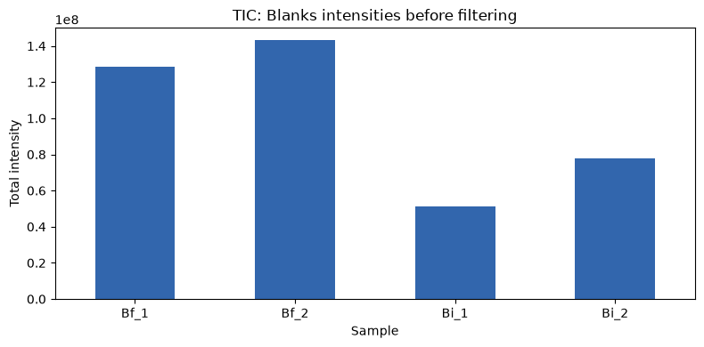
There is some signal. So we can run the blanks filtering, filtering out features with the default threshold.
data_blanks_05 = fm.filter_blanks(data, blanks=blanks, samples=samples)
Num. of features before filtering: 2545
Num. of features after filtering: 2275
Difference: 270 features removed.
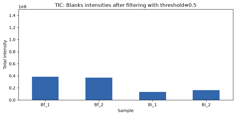
Keeping the y axis at the same scale, we can see that the total intensity has changed. Now we can check how it looks if we use a different parameter than the default.
data_blanks_01 = fm.filter_blanks(data, blanks=blanks, samples=samples, threshold=0.1)
Num. of features before filtering: 2545
Num. of features after filtering: 1862
Difference: 683 features removed.
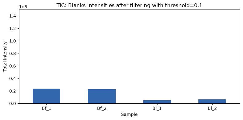
This threshold is more stringent so fewer features are retained which also means that there is less total intensity in the blanks samples.