

Imputation data (MS-example)#
We will explore imputation of proteomics data using an Alzheimer dataset where the data was collected in four different sites.
k Nearest Neighbour imputation can also be used with other types of data
the replacement from the normal distribution on the sample level is typical to normally distributed samples from mass spectrometer data (in the log2 space)
Refers to the acore.imputation_analysis module.
Common shared parameters across: imputation_KNN, imputation_normal_distribution and
imputation_mixed_norm_KNN function presented here:
data:pd.DataFramewith samples as rows and features as columns, which can can contain agroupcolumn.drop_cols: optional iterable of column names excluded from imputation.
%pip install acore vuecore
Set some parameters#
BASE = (
    "https://raw.githubusercontent.com/Multiomics-Analytics-Group/acore/"
    "main/example_data/alzheimer_proteomics/"
)
# data is already preprocessed: log2, filtered
fname: str = "alzheimer_example_omics_and_clinic.csv"  # combined omics and meta data
covariates: list[str] = ["age", "male"]
group: str = "collection_site"
subject_col: str = "Sample ID"
drop_cols: list[str] = ["AD"]
factor_and_covars: list[str] = [group, *covariates]
group_label: Optional[str] = "site"  # optional: rename target variable
Data loading#
Use combined dataset for ANCOVA analysis.
| AD | age | male | collection_site | Q6UX72 | O14773 | A0A0A0MQU6 | P36222 | P51693-2 | P17174 | ... | A0A075B6K4 | O15041 | J3KNA1 | A0A0C4DH33 | P16870 | G3V533 | Q9Y5I4 | P55283 | A1L4H1 | Q7Z4T9 | |
|---|---|---|---|---|---|---|---|---|---|---|---|---|---|---|---|---|---|---|---|---|---|
| Sample ID | |||||||||||||||||||||
| Sample_000 | 0 | 71 | 0 | Sweden | 16.047 | 18.412 | 16.381 | 20.948 | 18.658 | 20.232 | ... | 16.149 | 14.013 | 20.549 | 14.269 | 20.468 | 18.448 | 17.187 | 17.422 | 15.542 | 19.331 |
| Sample_001 | 1 | 77 | 1 | Sweden | 14.457 | 17.869 | 16.196 | 21.083 | 18.446 | 19.776 | ... | 16.127 | 13.916 | 15.854 | 14.379 | 19.902 | 17.723 | 17.447 | 17.097 | 15.734 | 18.980 |
| Sample_002 | 1 | 75 | 1 | Sweden | 15.631 | 17.662 | 16.071 | 21.206 | 18.967 | 20.066 | ... | 15.387 | 13.903 | 17.576 | 13.675 | 19.619 | 17.006 | 17.410 | 17.752 | 15.824 | 19.326 |
| Sample_003 | 1 | 72 | 0 | Sweden | 16.204 | 18.437 | 16.356 | 20.729 | 18.798 | 20.195 | ... | 16.565 | 14.526 | 18.173 | <NA> | 20.170 | 17.212 | 17.545 | 17.483 | 15.515 | 18.953 |
| Sample_004 | 1 | 63 | 0 | Sweden | 15.968 | 18.577 | 16.001 | 21.068 | 18.422 | 20.485 | ... | 16.418 | 14.933 | 15.440 | <NA> | 19.987 | 17.624 | 17.297 | 17.172 | 15.334 | 18.651 |
| ... | ... | ... | ... | ... | ... | ... | ... | ... | ... | ... | ... | ... | ... | ... | ... | ... | ... | ... | ... | ... | ... |
| Sample_205 | 1 | 69 | 0 | Berlin | 15.262 | 18.046 | 16.358 | 21.321 | 18.580 | 19.838 | ... | 15.350 | 13.572 | 13.482 | <NA> | 19.984 | 15.269 | 17.104 | 16.952 | 15.705 | 18.844 |
| Sample_206 | 0 | 73 | 1 | Berlin | <NA> | 16.573 | 16.099 | 20.663 | 19.191 | 18.388 | ... | 16.582 | 9.748 | 14.372 | 15.567 | 19.396 | 16.976 | 17.109 | 18.056 | 15.282 | 18.686 |
| Sample_207 | 0 | 71 | 0 | Berlin | 15.463 | 17.991 | 16.062 | 20.770 | 19.050 | 19.361 | ... | 15.768 | 13.241 | 13.931 | 15.092 | 19.923 | 16.669 | 16.938 | 17.248 | 14.874 | 19.146 |
| Sample_208 | 0 | 83 | 1 | Berlin | 15.786 | 17.216 | 15.929 | 20.938 | 18.216 | 19.183 | ... | 17.560 | 14.442 | <NA> | 14.267 | 19.831 | 16.258 | 17.155 | 16.353 | 15.471 | 16.853 |
| Sample_209 | 0 | 63 | 0 | Berlin | 15.691 | <NA> | 15.914 | 20.366 | 19.308 | 19.534 | ... | 16.338 | 13.628 | <NA> | 13.051 | 19.427 | 14.848 | 16.776 | 16.597 | 14.699 | 18.087 |
197 rows × 104 columns
Separate omics and the grouping variable
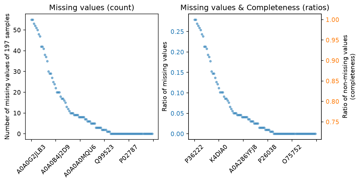
Show samples and features with at least 3 missing values
| Q6UX72 | O14773 | A0A0A0MQU6 | Q9BWS9 | A0A0B4J2D9 | Q13433 | P01258 | D6RJG0 | P48745 | Q10472 | ... | O60279 | P69905 | Q9BXJ3 | A0A075B6K4 | O15041 | J3KNA1 | A0A0C4DH33 | G3V533 | A1L4H1 | Q7Z4T9 | |
|---|---|---|---|---|---|---|---|---|---|---|---|---|---|---|---|---|---|---|---|---|---|
| Sample ID | |||||||||||||||||||||
| Sample_000 | 16.047 | 18.412 | 16.381 | 15.500 | 15.408 | 14.999 | 14.796 | <NA> | 17.516 | 16.143 | ... | 18.440 | 17.685 | 16.828 | 16.149 | 14.013 | 20.549 | 14.269 | 18.448 | 15.542 | 19.331 |
| Sample_001 | 14.457 | 17.869 | 16.196 | 14.760 | <NA> | 14.374 | 15.063 | <NA> | <NA> | 16.453 | ... | 18.305 | 17.978 | 16.793 | 16.127 | 13.916 | 15.854 | 14.379 | 17.723 | 15.734 | 18.980 |
| Sample_002 | 15.631 | 17.662 | 16.071 | <NA> | 15.362 | 15.121 | 14.219 | 16.359 | 16.870 | 16.097 | ... | 18.484 | 21.023 | 17.229 | 15.387 | 13.903 | 17.576 | 13.675 | 17.006 | 15.824 | 19.326 |
| Sample_003 | 16.204 | 18.437 | 16.356 | 15.300 | <NA> | 14.798 | 14.424 | 15.548 | 17.006 | 16.311 | ... | 18.381 | 16.445 | 16.886 | 16.565 | 14.526 | 18.173 | <NA> | 17.212 | 15.515 | 18.953 |
| Sample_004 | 15.968 | 18.577 | 16.001 | 16.054 | <NA> | 15.097 | 14.190 | <NA> | 17.316 | 16.188 | ... | 18.472 | 23.001 | 16.946 | 16.418 | 14.933 | 15.440 | <NA> | 17.624 | 15.334 | 18.651 |
| ... | ... | ... | ... | ... | ... | ... | ... | ... | ... | ... | ... | ... | ... | ... | ... | ... | ... | ... | ... | ... | ... |
| Sample_199 | 15.913 | 17.399 | 15.685 | 15.444 | <NA> | 12.306 | <NA> | <NA> | 17.841 | 16.002 | ... | 18.182 | 20.355 | 16.373 | 16.755 | 13.182 | 14.236 | <NA> | 16.024 | 14.467 | 18.661 |
| Sample_200 | 13.295 | <NA> | <NA> | 15.574 | 15.306 | <NA> | <NA> | 14.257 | 16.625 | 16.677 | ... | 17.712 | <NA> | <NA> | 18.582 | <NA> | <NA> | 16.537 | 17.281 | 15.432 | 18.273 |
| Sample_201 | 14.973 | 17.537 | 16.355 | 15.645 | 19.319 | <NA> | 13.310 | 16.158 | 16.649 | 16.946 | ... | 17.967 | 16.806 | 17.354 | 18.517 | <NA> | <NA> | 16.568 | 17.980 | 15.268 | 19.282 |
| Sample_206 | <NA> | 16.573 | 16.099 | 16.026 | 15.503 | <NA> | <NA> | 16.283 | 17.283 | 16.446 | ... | 18.202 | 15.514 | 17.000 | 16.582 | 9.748 | 14.372 | 15.567 | 16.976 | 15.282 | 18.686 |
| Sample_209 | 15.691 | <NA> | 15.914 | 15.653 | 13.784 | 13.923 | 13.667 | 16.084 | 16.659 | 16.680 | ... | 18.442 | 15.276 | 16.390 | 16.338 | 13.628 | <NA> | 13.051 | 14.848 | 14.699 | 18.087 |
132 rows × 58 columns
KNN imputation#
Can be generally applied
both by group and overall
returns the imputed data, per default only features that meet the criteria based on the selected cutoff for the fraction of non-missing values for a single feature (e.g. protein group).
setting
alone=Falsewill ensure that all features, imputed or not, are returned. This can be useful for downstream analysis where you want to keep all features, but only impute those that meet a minimal quality criteria.
overall#
cutoff = 0.60
omics_and_y_imputed = imputation_KNN(
    data=omics_and_y,
    drop_cols=[],
    group=None,
    cutoff=cutoff,
    alone=False,
)
assert omics_and_y_imputed.isna().sum().sum() == 0
omics_and_y_imputed
| Q6UX72 | O14773 | A0A0A0MQU6 | P36222 | P51693-2 | P17174 | Q9BWS9 | A0A0B4J2D9 | P00734 | Q13433 | ... | O15041 | J3KNA1 | A0A0C4DH33 | P16870 | G3V533 | Q9Y5I4 | P55283 | A1L4H1 | Q7Z4T9 | collection_site | |
|---|---|---|---|---|---|---|---|---|---|---|---|---|---|---|---|---|---|---|---|---|---|
| Sample ID | |||||||||||||||||||||
| Sample_000 | 16.047 | 18.412 | 16.381 | 20.948 | 18.658 | 20.232 | 15.500 | 15.408 | 19.870 | 14.999 | ... | 14.013 | 20.549 | 14.269 | 20.468 | 18.448 | 17.187 | 17.422 | 15.542 | 19.331 | Sweden |
| Sample_001 | 14.457 | 17.869 | 16.196 | 21.083 | 18.446 | 19.776 | 14.760 | 16.981 | 20.338 | 14.374 | ... | 13.916 | 15.854 | 14.379 | 19.902 | 17.723 | 17.447 | 17.097 | 15.734 | 18.980 | Sweden |
| Sample_002 | 15.631 | 17.662 | 16.071 | 21.206 | 18.967 | 20.066 | 14.635 | 15.362 | 19.814 | 15.121 | ... | 13.903 | 17.576 | 13.675 | 19.619 | 17.006 | 17.410 | 17.752 | 15.824 | 19.326 | Sweden |
| Sample_003 | 16.204 | 18.437 | 16.356 | 20.729 | 18.798 | 20.195 | 15.300 | 15.725 | 20.078 | 14.798 | ... | 14.526 | 18.173 | 14.462 | 20.170 | 17.212 | 17.545 | 17.483 | 15.515 | 18.953 | Sweden |
| Sample_004 | 15.968 | 18.577 | 16.001 | 21.068 | 18.422 | 20.485 | 16.054 | 15.833 | 19.786 | 15.097 | ... | 14.933 | 15.440 | 14.163 | 19.987 | 17.624 | 17.297 | 17.172 | 15.334 | 18.651 | Sweden |
| ... | ... | ... | ... | ... | ... | ... | ... | ... | ... | ... | ... | ... | ... | ... | ... | ... | ... | ... | ... | ... | ... |
| Sample_205 | 15.262 | 18.046 | 16.358 | 21.321 | 18.580 | 19.838 | 14.942 | 14.204 | 20.530 | 14.518 | ... | 13.572 | 13.482 | 16.096 | 19.984 | 15.269 | 17.104 | 16.952 | 15.705 | 18.844 | Berlin |
| Sample_206 | 15.217 | 16.573 | 16.099 | 20.663 | 19.191 | 18.388 | 16.026 | 15.503 | 21.106 | 13.421 | ... | 9.748 | 14.372 | 15.567 | 19.396 | 16.976 | 17.109 | 18.056 | 15.282 | 18.686 | Berlin |
| Sample_207 | 15.463 | 17.991 | 16.062 | 20.770 | 19.050 | 19.361 | 15.551 | 16.418 | 20.477 | 13.842 | ... | 13.241 | 13.931 | 15.092 | 19.923 | 16.669 | 16.938 | 17.248 | 14.874 | 19.146 | Berlin |
| Sample_208 | 15.786 | 17.216 | 15.929 | 20.938 | 18.216 | 19.183 | 15.176 | 14.104 | 20.483 | 13.929 | ... | 14.442 | 13.887 | 14.267 | 19.831 | 16.258 | 17.155 | 16.353 | 15.471 | 16.853 | Berlin |
| Sample_209 | 15.691 | 17.468 | 15.914 | 20.366 | 19.308 | 19.534 | 15.653 | 13.784 | 21.183 | 13.923 | ... | 13.628 | 13.919 | 13.051 | 19.427 | 14.848 | 16.776 | 16.597 | 14.699 | 18.087 | Berlin |
197 rows × 101 columns
As we have increased the threshold cutoff for the fraction of non-missing
values per feature, more features will not be imputed and therefore have
missing values.
cutoff = 0.90
omics_and_y_imputed = imputation_KNN(
    data=omics_and_y,
    drop_cols=[],
    group=None,
    cutoff=cutoff,
    alone=False,
)
n_still_missing = omics_and_y_imputed.isna().sum().sum()
print(f"Still missing features with cutoff of {cutoff}: {n_still_missing}")
Still missing features with cutoff of 0.9: 892
Keep only imputed features#
Use the alone=True to only keep the imputed features. It is the default.
cutoff = 0.90
omics_and_y_imputed = imputation_KNN(
    data=omics_and_y,
    drop_cols=[],
    group=None,
    cutoff=cutoff,
    alone=True,
)
assert omics_and_y_imputed.isna().sum().sum() == 0
print("Shape of of input data: ", omics_and_y.shape)
print("Shape of imputed data: ", omics_and_y_imputed.shape)
Shape of of input data:  (197, 101)
Shape of imputed data:  (197, 77)
By group#
Do the imputation separately for each group (e.g. target vs control) and then combine the results.
Let’s see the ratio of missing (left y-axis) and of non-missing (right y-axis) values per feature (e.g. protein group) for which no missing values for each group:
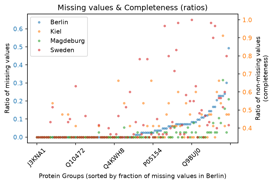
Clearly some protein groups only have missing values if combined from a certain collection site, and that the ratio can be different in each group. Therefore, imputation by KNN for a threshold of non-missing values per feature (e.g. protein group) per group can be a good option.
omics_and_y_imputed = imputation_KNN(
    data=omics_and_y,
    drop_cols=[],
    group=group,
    cutoff=0.65,  # selected to leave some missing values for demonstration
    alone=False,
)
omics_and_y_imputed.isna().sum().value_counts().sort_index()
0    87
9     1
22    1
26    2
27    2
29    1
33    1
37    2
38    2
39    1
41    1
Name: count, dtype: int64
If we look at the number of missing values still remaining by collection site, we see that Sweden has most of these missing values due to a higher fraction of missing values for these.
Berlin  Kiel  Magdeburg  Sweden
0       0     0          0        86
                         22        1
                         26        2
                         27        2
                         29        1
                         33        1
                         37        2
                         38        2
                         39        1
        9     0          0         1
41      0     0          0         1
Name: count, dtype: int64
As we increase the threshold cutoff for the fraction of non-missing
values per feature, more features will not be imputed and therefore have
missing values.
omics_and_y_imputed = imputation_KNN(
    data=omics_and_y,
    drop_cols=[],
    group=group,
    cutoff=0.90,
    alone=False,
)
n_still_missing = omics_and_y_imputed.isna().sum().sum()
print(f"Still missing features with cutoff of {cutoff}: {n_still_missing}")
Still missing features with cutoff of 0.9: 927
Imputation from a shifted normal distribution per sample#
Specific to massspectrometry based data in log2 space: normal distributed data, with detection limit (if that applies it can be used)
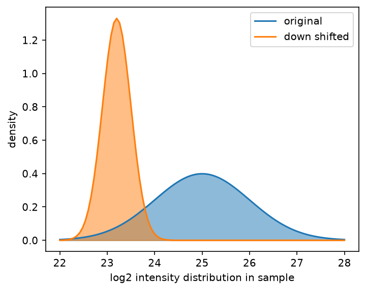
based on mean and standard deviation missing values are replaced by drawing random values from a shifted normal distribution
assumption is that missing values are due to falling below the detection limit which can be revealed by the distribution of intensities
Below you find a generated example highlighting the idea
Downshifted: mu_shifted = 23.2, stddev_shifted = 0.3
This idea can be applied on a per sample basis using:
# does not account for groups as it is done on a per sample basis (along columns)
imputation_normal_distribution(
    data=omics_and_y,
    drop_cols=[group],
)
| Q6UX72 | O14773 | A0A0A0MQU6 | P36222 | P51693-2 | P17174 | Q9BWS9 | A0A0B4J2D9 | P00734 | Q13433 | ... | A0A075B6K4 | O15041 | J3KNA1 | A0A0C4DH33 | P16870 | G3V533 | Q9Y5I4 | P55283 | A1L4H1 | Q7Z4T9 | |
|---|---|---|---|---|---|---|---|---|---|---|---|---|---|---|---|---|---|---|---|---|---|
| Sample ID | |||||||||||||||||||||
| Sample_000 | 16.047 | 18.412 | 16.381 | 20.948 | 18.658 | 20.232 | 15.500 | 15.408 | 19.870 | 14.999 | ... | 16.149 | 14.013 | 20.549 | 14.269 | 20.468 | 18.448 | 17.187 | 17.422 | 15.542 | 19.331 |
| Sample_001 | 14.457 | 17.869 | 16.196 | 21.083 | 18.446 | 19.776 | 14.760 | 11.019 | 20.338 | 14.374 | ... | 16.127 | 13.916 | 15.854 | 14.379 | 19.902 | 17.723 | 17.447 | 17.097 | 15.734 | 18.980 |
| Sample_002 | 15.631 | 17.662 | 16.071 | 21.206 | 18.967 | 20.066 | 12.206 | 15.362 | 19.814 | 15.121 | ... | 15.387 | 13.903 | 17.576 | 13.675 | 19.619 | 17.006 | 17.410 | 17.752 | 15.824 | 19.326 |
| Sample_003 | 16.204 | 18.437 | 16.356 | 20.729 | 18.798 | 20.195 | 15.300 | 12.219 | 20.078 | 14.798 | ... | 16.565 | 14.526 | 18.173 | 12.783 | 20.170 | 17.212 | 17.545 | 17.483 | 15.515 | 18.953 |
| Sample_004 | 15.968 | 18.577 | 16.001 | 21.068 | 18.422 | 20.485 | 16.054 | 12.687 | 19.786 | 15.097 | ... | 16.418 | 14.933 | 15.440 | 12.722 | 19.987 | 17.624 | 17.297 | 17.172 | 15.334 | 18.651 |
| ... | ... | ... | ... | ... | ... | ... | ... | ... | ... | ... | ... | ... | ... | ... | ... | ... | ... | ... | ... | ... | ... |
| Sample_205 | 15.262 | 18.046 | 16.358 | 21.321 | 18.580 | 19.838 | 14.942 | 14.204 | 20.530 | 14.518 | ... | 15.350 | 13.572 | 13.482 | 12.086 | 19.984 | 15.269 | 17.104 | 16.952 | 15.705 | 18.844 |
| Sample_206 | 14.085 | 16.573 | 16.099 | 20.663 | 19.191 | 18.388 | 16.026 | 15.503 | 21.106 | 11.743 | ... | 16.582 | 9.748 | 14.372 | 15.567 | 19.396 | 16.976 | 17.109 | 18.056 | 15.282 | 18.686 |
| Sample_207 | 15.463 | 17.991 | 16.062 | 20.770 | 19.050 | 19.361 | 15.551 | 12.091 | 20.477 | 13.842 | ... | 15.768 | 13.241 | 13.931 | 15.092 | 19.923 | 16.669 | 16.938 | 17.248 | 14.874 | 19.146 |
| Sample_208 | 15.786 | 17.216 | 15.929 | 20.938 | 18.216 | 19.183 | 15.176 | 14.104 | 20.483 | 13.929 | ... | 17.560 | 14.442 | 10.987 | 14.267 | 19.831 | 16.258 | 17.155 | 16.353 | 15.471 | 16.853 |
| Sample_209 | 15.691 | 11.367 | 15.914 | 20.366 | 19.308 | 19.534 | 15.653 | 13.784 | 21.183 | 13.923 | ... | 16.338 | 13.628 | 9.967 | 13.051 | 19.427 | 14.848 | 16.776 | 16.597 | 14.699 | 18.087 |
197 rows × 100 columns
Note that using this type of imputation before differential regulation can lead to false positive and negative results. If values are not due to assumed missing mechanism (Missing not-at-random due to low abundance), but are due to technical noise, these values should not be replaced.
Therefore, in proteomics, many use a combined approach Santos et al., 2020:
Combining KNN based imputation and random imputation from a shifted random distribution#
For features (e.g. protein groups) that are present across groups in high enough frequency, use KNN-based imputation (which is deterministic)
for the remaining missing values, use - based on the distribution of observed values in a sample - a shifted normal distribution to draw replacements (random, but deterministic due to the set seed).
See the methods section of Santos et al., 2020 for more details.
imputation_mixed_norm_KNN(data=omics_and_y, drop_cols=[], group=group, cutoff=0.9)
| Q6UX72 | O14773 | A0A0A0MQU6 | P36222 | P51693-2 | P17174 | Q9BWS9 | A0A0B4J2D9 | P00734 | Q13433 | ... | A0A075B6K4 | O15041 | J3KNA1 | A0A0C4DH33 | P16870 | G3V533 | Q9Y5I4 | P55283 | A1L4H1 | Q7Z4T9 | |
|---|---|---|---|---|---|---|---|---|---|---|---|---|---|---|---|---|---|---|---|---|---|
| Sample ID | |||||||||||||||||||||
| Sample_000 | 16.047 | 18.412 | 16.381 | 20.948 | 18.658 | 20.232 | 15.500 | 15.408 | 19.870 | 14.999 | ... | 16.149 | 14.013 | 20.549 | 14.269 | 20.468 | 18.448 | 17.187 | 17.422 | 15.542 | 19.331 |
| Sample_001 | 14.457 | 17.869 | 16.196 | 21.083 | 18.446 | 19.776 | 14.760 | 12.534 | 20.338 | 14.374 | ... | 16.127 | 13.916 | 15.854 | 14.379 | 19.902 | 17.723 | 17.447 | 17.097 | 15.734 | 18.980 |
| Sample_002 | 15.631 | 17.662 | 16.071 | 21.206 | 18.967 | 20.066 | 11.854 | 15.362 | 19.814 | 15.121 | ... | 15.387 | 13.903 | 17.576 | 13.675 | 19.619 | 17.006 | 17.410 | 17.752 | 15.824 | 19.326 |
| Sample_003 | 16.204 | 18.437 | 16.356 | 20.729 | 18.798 | 20.195 | 15.300 | 12.244 | 20.078 | 14.798 | ... | 16.565 | 14.526 | 18.173 | 11.338 | 20.170 | 17.212 | 17.545 | 17.483 | 15.515 | 18.953 |
| Sample_004 | 15.968 | 18.577 | 16.001 | 21.068 | 18.422 | 20.485 | 16.054 | 12.632 | 19.786 | 15.097 | ... | 16.418 | 14.933 | 15.440 | 11.061 | 19.987 | 17.624 | 17.297 | 17.172 | 15.334 | 18.651 |
| ... | ... | ... | ... | ... | ... | ... | ... | ... | ... | ... | ... | ... | ... | ... | ... | ... | ... | ... | ... | ... | ... |
| Sample_205 | 15.262 | 18.046 | 16.358 | 21.321 | 18.580 | 19.838 | 14.942 | 14.204 | 20.530 | 14.518 | ... | 15.350 | 13.572 | 13.482 | 12.789 | 19.984 | 15.269 | 17.104 | 16.952 | 15.705 | 18.844 |
| Sample_206 | 15.474 | 16.573 | 16.099 | 20.663 | 19.191 | 18.388 | 16.026 | 15.503 | 21.106 | 12.437 | ... | 16.582 | 9.748 | 14.372 | 15.567 | 19.396 | 16.976 | 17.109 | 18.056 | 15.282 | 18.686 |
| Sample_207 | 15.463 | 17.991 | 16.062 | 20.770 | 19.050 | 19.361 | 15.551 | 15.776 | 20.477 | 13.842 | ... | 15.768 | 13.241 | 13.931 | 15.092 | 19.923 | 16.669 | 16.938 | 17.248 | 14.874 | 19.146 |
| Sample_208 | 15.786 | 17.216 | 15.929 | 20.938 | 18.216 | 19.183 | 15.176 | 14.104 | 20.483 | 13.929 | ... | 17.560 | 14.442 | 12.303 | 14.267 | 19.831 | 16.258 | 17.155 | 16.353 | 15.471 | 16.853 |
| Sample_209 | 15.691 | 12.638 | 15.914 | 20.366 | 19.308 | 19.534 | 15.653 | 13.784 | 21.183 | 13.923 | ... | 16.338 | 13.628 | 11.662 | 13.051 | 19.427 | 14.848 | 16.776 | 16.597 | 14.699 | 18.087 |
197 rows × 100 columns
done.